Tutorial: PALEOMAP PaleoAtlas for GPlates and the PaleoData Plotter Program

http://www.earthbyte.org/paleomap-paleoatlas-for-gplates/ by

Christopher R. Scotese, PALEOMAP Project February 16, 2016

Abstract

This report describes the contents of the PALEOMAP PaleoAtlas for GPlates, describes how the maps in the PaleoAtlas were made, documents the sources of information used to make the paleogeographic maps, and provides instructions how to plot user-defined paleodata on the paleogeographic maps using the program “PaleoDataPlotter”. The PALEOMAP PaleloAtlas and the program (Mac OSX) can be downloaded at http://www.earthbyte.org/paleomap paleoatlas-for-gplates/ .

Please cite this work as: Scotese, C.R., 2016. PALEOMAP PaleoAtlas for GPlates and the PaleoData Plotter Program, PALEOMAP Project, http://www.earthbyte.org/paleomap paleoatlas-for-gplates/

Part I. Introduction

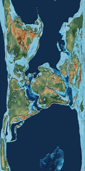
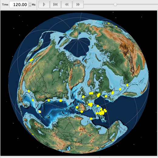
The PALEOMAP PaleoAtlas for GPlates consists of 91 paleogeographic maps spanning the Phanerozoic and late Neoproterozoic. Table 1 lists all the time intervals that comprise the six volumes of the PALEOMAP PaleoAtlas for GPlates. The PaleoAtlas contains one map for nearly every stage in the Phanerozoic, as well as 3 maps for the late Precambrian. The PaleoAtlas can be directly loaded into GPLates as a “Time Dependant Raster” file (see Part III, “Loading the PALEOMAP PaleoAtlas into GPlates”). A paleogeographic map is defined as a map that shows the ancient configuration of the ocean basins and continents, as well as important topographic and bathymetric features such as mountains, lowlands, shallow sea, continental shelves, and deep oceans (Figure 1, Early Cretaceous, 121.8 Ma). Ideally, a paleogeographic map would be the kind of reference map that any time traveler would like to have before embarking on a journey back through time.

Colorful paleogeographic maps may be nice to look at, but the maps become much more useful for research and teaching purposes if users can plot their own data on the maps.

In this regard, user-defined paleodata can be plotted on the paleogeographic maps in two ways: 1) using GPLates tools and procedures to import symbols and labels in a GIS-format (see GPlates Tutorial 1.1: Loading and Saving Data), and 2) by loading user-defined, latitude/longitude point data “text files” using the program “PaleoDataPlotter”. The latter method is described in the Section IV, “Plotting User-Defined Data on the Paleogeographic Reconstructions”.

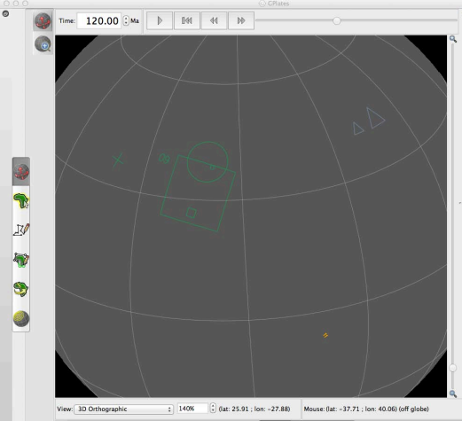
PaleoDataPlotter, which is provided with this report, creates a variety of geometric symbols (circles, squares, triangles, stars, plus signs, crosses, small dots, and arrows) as well as short numeric labels (up to 5 digits), that can be plotted on the paleogeographic map at user-defined latitude/longitude coordinates (Figure 2). The PaleoDataPlotter program is ideal for plotting fossil localities, geological outcrops, as well as the locations of drill sites, wells, stratigraphic sections, or any point data set whose geographic location can be specified by modern, latitude and longitude coordinates. The arrow symbol, which can be oriented according to a user-supplied azimuth, is particularly useful for plotting “vector” information such as: ocean current directions, river flow, wind directions, paleomagnetic declinations, stress fields, and instantaneous plate motions. In a future version, the PaleoDataPlotter will also be able to plot text-labels at specific latitude/longitude coordinates.

Part II. How the Paleogeographic Maps were Made: The Paleogeographic Method

Some of you may want to know how the paleogeographic maps were made. In this section, I briefly discuss the geologic and geophysical data that were used to make the maps and describe the methodology that was followed to reimagine the paleotopography and paleobathymetry, (i.e. the paleogeography).

The paleogeographic maps in the GPlates version of the PALEOMAP PaleoAtlas were originally published in the PALEOMAP PaleoAtlas for ArcGIS (Scotese, 2008a-f). This digital atlas, designed for use with GIS software, (ArcMap, ESRI), consists of ~100 paleogeographic maps together with plate tectonic (Scotese, 2014f), paleolithological (Boucot et al., 2013), paleoceanographic (Scotese, 2014a; Scotese and Moore, 2014a,e), and paleoclimatic

reconstructions (Scotese et al., 2014; Scotese and Moore, 2010, 2014b,c,d) . The original paleogeographic maps, which can be viewed in the folder, (“PALEOMAP_PaleoAtlas.zip”), have been saved as jpg images (3600 x 1800 pixels) in a rectilinear projection. A rectilinear projection (i.e., Cartesian latitude and longitude) was used because a rectilinear map can be directly “wrapped” onto a 3D spherical projection, like the one used in GPlates.

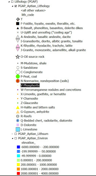
Once a global plate tectonic framework has been established (Scotese and Sager, 1988; Scotese, 1990; Scotese and McKerrow, 1990; Scotese, 2001; Scotese and Dammrose, 2008, Scotese, 2014b, Scotese, 2016), paleogeographic maps that represent the ancient distribution of highlands, lowlands, shallow seas, and deep ocean basins can be digitally constructed. This is done is several steps. The first step is to map the geological lithofacies that define the ancient depositional environments (Figure 3). For example, a thick sequence of pure limestones might represent warm, shallow water environments like the Bahamas Platform or vast a epeiric sea. Extensive sets of massive, cross-bedded sandstones may once have been wind-blown, desert dunes. A terrane composed of andesite and granodiorite may have been a continental arc or Andean mountain range. Table 2 summarizes the lithofacies and rock types that correspond to the depositional environments that have been used to interpret the ancient topography and bathymetry. There is nothing complex or mysterious about this procedure. It’s mostly data collection and mapping, i.e. basic geology.

Geologists have been collecting lithologic information and producing lithofacies and paleoenvironmental maps for more than 200 years (William Smith, 1815). During the late 1970’s and early 1980’s, the Paleogeographic Atlas Project, under the leadership of Prof. A. M. Ziegler, in the Department of Geophysical Sciences, University of Chicago, compiled a data base of more than 125,000 lithological and paleoenvironmental records for the Mesozoic and Cenozoic (Ziegler, 1975; Ziegler and Scotese, 1977; Ziegler et al., 1985). This database was supplemented by additional lithological and paleoenvironmental records for the Permian and Jurassic (Rees et al., 2000; 2002). These two datasets, in combination with numerous regional and global paleogeographic atlases, were used to construct the paleogeographic maps that appear in the PALEOMAP PaleoAtlas. See Table 4 for a list of key paleogeographic compilations and atlases.

Lithofacies can be used to map paleogeographic environments where only the rock record is fairly complete. However, there are many instances where the rock record has

been eroded, destroyed by tectonic processes, or covered by younger strata. For these areas, a second, more interpretive approach needs to be taken to restore the paleogeography. (This is where the fun begins!) In these instances the paleoenvironments and paleogeography must be inferred from the tectonic history of a region. The PALEOMAP Global Plate Tectonic Model (Scotese, 2016), provides the tectonic framework required to make these inferences and interpretations. The plate tectonic reconstructions (Scotese, 2014a) are used to “model” the expected changes in topography and bathymetry caused by plate tectonic events, such as: sea floor spreading, continental rifting, subduction along Andean margins, and continental collision, as well as other isostatic events such as glacial rebound (Peltier, 2004). For example, to produce a paleogeographic map for the early Cretaceous, young tectonic features, such as recent uplifts or volcanic eruptions (e.g. Mid African Rift), must be removed or reduced in size, whereas older tectonic features, such as ancient mountain ranges (e.g. Appalachian mountians), must be restored to their former extent. This approach is similar to the techniques described by Verard et al. (2015) and Baatsen et al. (2015).

In a similar manner, the paleobathymetry of the ocean floor must be restored back through time. Oceanic lithosphere is produced at mid-ocean ridges. As ocean floor moves away from the spreading ridge, it cools and subsides. In many respects restoring the past bathymetry of the ocean floor is much easier than estimating the elevation of ancient

mountain ranges (Rowley et al., 2001; 2006; 2007). This is because as the ocean floor ages, it cools. As it cools, it sinks. The amount that it sinks through time follows a regular mathematical rule that states that the amount of thermal subsidence is inversely proportional to the square root of the age of the oceanic crust (Parsons and Sclater, 1977). To restore the ancient ocean floor to its former depths, the bathymetry of the ocean floor was “unsubsided” using the depth/age relationship published by Stein and Stein (1992).

Once the paleogeography for each time interval has been mapped and the corrections to the topography and bathymetry have been duly noted, this information is then converted into a digital representation of paleotopography and paleobathymetry. Each paleogeographic map is composed of over 6 million grid cells that capture digital elevation information at a 10 km x 10 km horizontal resolution and 40 meter vertical resolution. This quantitative, paleo-digital elevation model, or “paleoDEM”, allows us to visualize and analyze

the changing surface of the Earth through time using GIS software and other computer modeling techniques.

The process of building a paleoDEM (Scotese, 2002) begins with digital topographic and bathymetric data sets of the modern world (Smith and Sandwell, 1997), Antarctica (Lythe and Vaughan, 2000), and the Arctic, (Jakobsson et al., 2004). These topographic and bathymetric data sets are combined into a global data set with 6-minute resolution. In the next step, the individual grid cells (latitude, longitude) are rotated back to their paleopositions using the global plate tectonic model of the PALEOMAP Project (Scotese, 2016). The resulting map is a reconstruction of present-day bathymetry and topography in a paleolatitudinal and paleolongitudal framework – not very interesting or informative, but a starting point!

In the next processing steps (Scotese, 2002), the modern digital topographic and bathymetric values are corrected and modified using the lithofacies and paleoenvironmental information described in the previous section. This is done using modern analogs for ancient geographies, and simple computer graphics techniques. In this step the digital evelation information is converted to “grayscale” values, where white (grayscale value = 255) represents the highest elevations and black (grayscale value=0) represents the deepest ocean trenches. Using 256 grayscale values it is possible to map the topography and bathymetry at a resolution of 40 meters, vertically. There are fewer grayscale values for high mountains and deep trenches because these regions represent only a small portion of the Earth’s surface.

To increase or decrease the elevation of a pixel, it becomes simply a matter of changing the grayscale values until the digital model matches the paleoenvironment or a modern analog. For example, the modern topography for the East African Rift was produced during the last 30 million years. Therefore, on a late Eocene (35 Ma) paleogeographic map of East Africa, the modern topography of the East African Rift must be “erased”. This is accomplished by digitally editing the mountainous grayscale values and replacing them with the grayscale values that represent lowlands and plains. Conversely, an area that was once was an ancient rift valley, but has been eroded flat, can be “rejuvenated” by replacing them with grayscale values that represent highlands. A reasonable way to do this is to use the modern topography as an analog. For example, the detailed “continental rift” topography in

the proto-South Atlantic region shown in Figure 1, was actually “cloned” from portions of the East African Rift.

In either case, recreating ancient topographic features requires a thorough understanding of the overall tectonic evolution of a region, as well as the precise knowledge of the tectonic history of every important geographic feature. One must be able to answer questions like: “When did this geographic feature first appear?”, “How long did it remain an important geographic feature?”, “When was it eroded?”. It is also important to note that any changes made on one map must be consistent with the preceding map, as well as, with subsequent paleogeographies. That is to say, tectonic features don’t suddenly appear and disappear. In fact the best overall strategy, when building the paleotopographic models, is to start at the present-day geography and work systematically backwards though time, map by map, undoing most recent tectonic events and gradually recreating ancient tectonic features.

Continuing with our discussion of the methodology of producing a paleogeographic model, once the grayscale version of the paleoelevations has been completed, then the grayscale values can be converted back to digitial elevation values. The resulting digital elevation file is a “revised” global paleotopographic and paleobathymetric surface, or paleoDEM, that represents the elevation of the land surface and the depth of the ocean basins for a specific geological time interval.

To complete the 3D paleogeographic model and produce a map that shows the location of the paleocoastline (the most important paleoenvironmental feature), the new topographic surface is digitally “flooded” by raising or lowering sea level according to the estimates from various eustatic sea level curves (Haq et al., 1987; Haq and Schutter, 2009; Ross and Ross, 1985; Miller et al., 2005). We have found that eustatic sealevel changes that are ~33% less than the values published by Haq et al. (1987) produce the best match between predicted continental flooding and the geological evidence of ancient shallow seas.

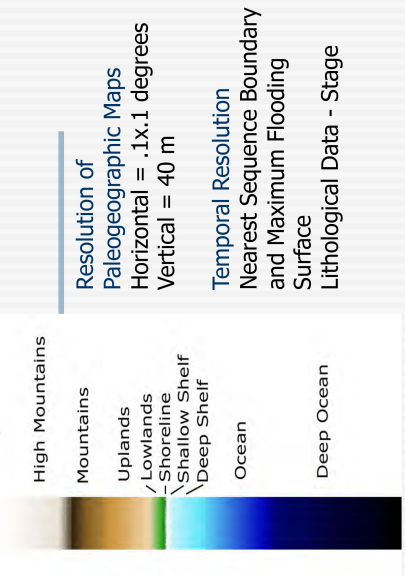
To complete the paleogeographic reconstruction, each grid-cell in the paleo-digitial elevation model (PaleoDEM) is given a unique color based on its depth or elevation (-10,000 meters below sea level to +10,000 meters above sea level). Deep oceans (oceanic crust) - dark blue. Mid-ocean ridges - blue. The shallow shelves and the flooded portions of the continents (epieric seas) - shades of light blue. Coastal regions and continental areas near sea level - dark green; low-lying inland areas - green. Plateaus and the foothills of mountains

- tan, and mountainous regions - brown. The highest peaks in the mountains - shaded white (Figure 4).

Part III. Loading the PALEOMAP PaleoAtlas into GPlates

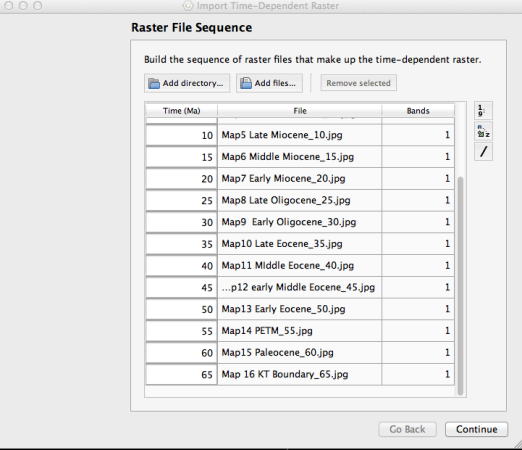
The PALEOMAP PaleoAtlas is composed of six volumes: Cenozoic, Cretaceous, Jurassic & Triassic, Late Paleozoic, Early Paleozoic and Late Precambrian (Scotese, 2008a-f). Each volume has ~15 individual paleogeographic maps (jpg images), one for each geological stage (approximately one map every 5 million years). These jpg images are loaded into GPlates using the “Import Time Dependent Raster” procedure.

To load the PALEOMAP PaleoAtlas into GPlates, follow these steps:

• Download the PaleoAtlas files from: http://www.earthbyte.org/paleomap paleoatlas-for-gplates/

• Open GPlates

• Go to the “File Menu”.

• Select “Import” and select “Import Time Dependent Raster” from the drop down menu.

• The “Raster File Sequence” page should appear.

• Click-on the “add directory box” (highlighted in blue) and navigate your directory to find the folder “PALEOMAP PaleoAtlas Rasters”.

• Select “Choose” (lower-left corner).

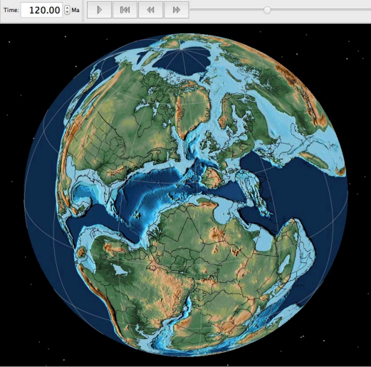
• After a few seconds a spinning colored ball will appear, it takes ~ 20-30 seconds to load all the maps (be patient). The display should look like this (Figure 5). • On the next few pages click, “Continue”, “Continue”, “Continue”, and “Done “. • You have successfully created a “gpml” version of the PALEOMAP PaleoAtlas called “PALEOMAP PaleoAtlas.gpml”. “gpml” is the native file format used with GPLates. • All the maps that comprise the PALEOMAP PaleoAtlas (should now appear on the screen. You can scroll through the maps using the “time scroll bar” at the top of the page (Figure 6).

Note: To view the older maps, be sure to enter 750 (million years) into the time box in the upper left-hand corner of the GPlates home screen.

Note: You need to follow the instructions given above, only once; i.e., the first time you load the PALEOMAP PaleoAtlas raster images. For all subsequent uses of the PaleoAtlas all you need to do is load the “gpml” file that you created. The “gpml” file should be located in the same file folder as the jpg images.

Part IV. Plotting User-Defined Data on the Paleogeographic Reconstructions

In order to help geologists, paleontologists, and paleomagnetists reconstruct and visualize the data sets that they routinely use, I have written a program called “PaleoDataPlotter” that creates a variety of geometric symbols (circles, squares, triangles, stars, plus signs, crosses, small dots, and arrows), as well as short alphanumeric labels (up to 8 characters) that can be plotted on the paleogeographic maps at user-defined latitude/longitude coordinates (Figure 2).

There are several ways to do this in GPlates, but only if you know how to import the labels and symbolic information from an ArcGIS program such as ArcGIS (ESRI) or QGIS in the “shapefile” format. For those who are less GIS-proficient, the PaleoDataPlotter (PDP) program allows you to create labels and symbols from simple text files or spreadsheets that contain the information describing the type of symbol and its size. What’s required is the modern latitude and longitude coordinates of the label or symbol, the symbol type, and its size. Using the PaleoData Plotter any user can plot and reconstruct a variety of symbols on the paleogeographic maps or other plate tectonic reconstructions produced by GPlates. The PaleoDataPlotter program is located in the download file called

“PaleoDataPlotter_Program”. This zipped archive also contains a set of sample input files: AptianReefs_URN.csv, AptianReefs.csv, AptianReefs_URN.csv, and

ExampleSymbolParametersFile.csv

PaleoDataPlotter generates outputfiles in a text-readable, if somewhat archane, format called “.dat” format that I developed when I was a graduate to input a variety of point, line, and polygon data for my reconstructions.

The PaleoData Plotter program is ideal for plotting fossil localities, geological outcrops, as well as the locations of drill sites, wells, stratigraphic sections, or any point data set whose geographic location is defined by modern latitude and longitude coordinates. The arrow symbol, which can be oriented according to a user-supplied azimuth, is particularly useful for plotting “vector” information such as: ocean current directions, river flow, wind directions, paleomagnetic declination, stress fields, and instantaneous plate motions (See Sample User Session).

How to make symbols and numeric labels for PaleoData.

To make your own symbols for your PaleoData, just follow these 4 steps.

Step 1. Build Symbol Parameter File

The first step is to build a simple text file that has all the necessary information. This file is called the “symbol parameter file”, because, as you may have guessed, it contains all the parameters need to generate the symbols or labels. I would recommend using Excel to generate your symbol parameter file and saving the file in “.csv” (comma-delimited) format. You can use a text editor or a word processing program to build the comma-delimited file, but you may run into problems if the editor or word processing program, unbeknownst to you, adds hidden characters or the wrong end-of-line terminator. (This drove me crazy for about two weeks.)

This symbol parameter file.csv contains the information that PaleoDataPlotter needs to build the “SymbolLabel.dat” file that you will load into GPlates. Two example symbol parameter files have been included with this tutorial. “ExampleSymbolParameterFile.csv” plots the rando assortment of symbols shown in Figure 2. “AptianReefs.csv” plots the location of early Cretaceous reefs (Kiessling et al., 2002) shown in Figures 9 &10. You can use these files as a starting point to build your own files.

Here are the first few lines of a very simple “.csv” input file:

Line 1 - URN, Label, PlateId,Latitude,Longitude,SymbolOrNumericLabel, Size, Azimuth

Line 2 - 1,Chicago,101,43,-87,circle,1,0

Line 3 - 2,Big Easy,101,30,-90,square,2,0

Line 4 - 3,London,301,50,0,triangle,1.5,0

Line 5 - 4,LA,101,42, -118,label,2,0

Line 6 - 5,Sydney,801,34,-144,arrow,1,90

It’s probably pretty obvious what all these fields and values mean, but let me describe them in a bit more detail.

The first line of the spreadsheet lists the “field” names. There eight required field names:

“URN, Label, PlateId, Latitude, Longitude, SymbolOrNumericLabel, Size, Azimuth “

Note that I said required, not “optional”. Do not leave out any field or change the order of the fields. If you make any changes or leave something off, the program won’t work.

Field definitions:

URN - URN stands for unique record number. When you build a dataset, it’s a good idea to give each record in that data set a “unique record number”. That way you can find it or identify it, if it goes missing. It must be an integer numeric string, with a maximum of five numbers (e.g., 2, 45, 234,78236).

Label - Label is a short description. It will be stored as an alphanumeric string. PlateID – The PlateID connects your data to the rotation model in GPlates. The data will not reconstruct if you do not have a PlateID. You can explicitly give each symbol/label a PlateID in this input file or you can let GPlates assign the PlateID. If you choose the second option, then you can enter a default PlateID of 999. A little bit later in this User’s Guide I will describe how to assign PlateID’s using GPlates.

Latitude - This is a number between 90.0 and -90.0 that describes the latitude of your site. Positive numbers are northern hemisphere, negative numbers are southern hemisphere. You must provide decimal values – no minutes and seconds nonsense.

Longitude - This is a number between 180.0 and -180.0 that describes the longitude of your site. Positive numbers are eastern hemisphere, negative numbers are western hemisphere. You must provide decimal values – no minutes and seconds nonsense.

SymbolOrNumericLabel – This is where you tell PaleoDataPlotter what kind of symbol you want, or if you are plotting a label. If you want a symbol enter one of these: circle, square, triangle, star, plus, cross, dot, or arrow. “Plus” is a plus sign. “Cross” is an “X”. And I’m sorry. I know some of you out there would have really liked to have hexagons, dodecagons, exclamation points, @-signs and asterisks. Maybe in the next version (not).

If you want to use the number in the “URN” field as a numeric label on the paleoglobe, simply enter “URN” in this field. The file “AptianReefs_URN.csv” has been included as an example of how to build a “labels” file for your data localities.

Size - The size of the symbol or label is the north-south distance measured in degrees. A value of “1” will generate a symbol or a label that is one degree high. If you generate really large symbols or labels (>30 degrees), they will begin to get a little wonky. (Why would you want to do that anyway?) Otherwise the symbols will remain undistorted on a sphere, and mostly undistorted in the various flat map projections (except near the poles).

Finally,

Azimuth - This is a value from 0 to 360 that allows you to spin your symbol or label about it’s center. It’s mostly used for arrows, can be creatively used to make “upside-down triangles” or turn squares in “diamonds”. Do not leave this field blank. The program is expecting a value, even if that value is “0”.

Notes:

1. If you have any questions, have a look at the “.csv” files that were included with this user-guide.

2. The “.csv” suffix may not automatically immediately appear when you save your Excel file. You may have to scroll down through the output formats to find it.

Step 2. Run PaleoDataPlotter

Now that you have built your “SymbolParameterFile.csv”. Now it’s time to run “PaleoDataPlotter”. (Unfortunately, the PaleoDataPlotter runs only under Apple OS X.) To run “PaleoDataPlotter”, follow these steps:

• Find the “PaleoDataPlotter” executable. It should be in folder “ PaleoAtlas for GPlates”.

• Double click on the icon “PaleoDataPlotter” to run it.

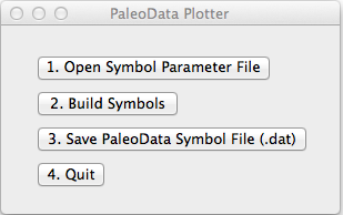
• A small window should open with four buttons, labeled: “1. Open Symbol Parameter File, 2. Build Symbols, 3. Save File, 4. Quit.” (see Figure 7).

• Click-on Button “1. Open Symbol Parameter File”. A New window should open up. Navigate the file directory and find the symbol parameter file that you created in Step 1. Click “Open” in the lower left-hand corner of the window.

• Click-on Button “2. Build Symbols”. A message box should appear telling you that the program has successfully run.. Click-on “OK” to close the message box. • Click-on Button “3. Save PaleoData Symbol File in .dat Format”. “Save” window should appear. Give the file a name and save it to a folder of your choosing. IMPORTANT: Be sure to add the “.dat” extension to the file name (no quotes). GPlates will only be able to read the PaleoData Symbol File, if it ends in the .dat extension. • Click-on “4. Quit”

Step 3. Load PaleoData Symbol File into GPlates

You’ve done most of the hard stuff. Now let’s look at your PaleoData Symbol File in GPlates.

To load your PaleoData Symbol File in GPlates, follow these steps:

• Open GPlates

• Go to the “File” menu and select “Open Feature Collection . . .”. A New window should open up. Navigate the file directory and find the PaleoData Symbol File (.dat) that you created in Step 2. Click “Open” in the lower left-hand corner of the window.

• The symbols that you created for your PaleoData Symbols should appear on the globe display in GPlates (Figure 4).

•

Step 4. Assign PlateIds so that The PaleoData Symbols will reconstruct with the continents. You can skip this step if you knew the correct PlateIds and included them in the symbol parameter file described in Step 1. If you didn’t know the correct PlateId for each

locality, you can let GPlates assign the PlateIds by following these steps. (A more detailed description of this procedure is given in GPlates Tutorial 1.5: Creating Features.) • Open GPlates

• Open your Paleodata Symbol File (.dat)

• Open the global plate polygon file provided by GPlates . This will be your “cookie cutter”. Note: If you want to plot your data localities on the raster maps of the PALEOMAP PaleoAtlas then you must open the “PALEOMAP PlatePolygons.gpml “cookie-cutter”, and the “PALEOMAP PlateModel.rot” (in the PALEOMAP Global Plate Model folder). • Go to the “Features” menu and select “Assign Plate IDs . . .”

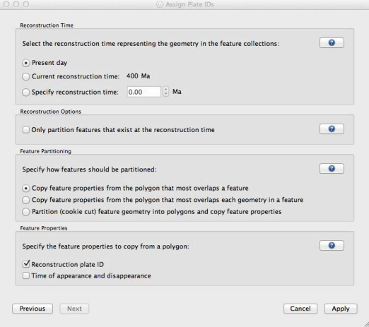
• Select the plate polygon file as the “partitioning layer” and hit “Next”. • Select the PaleoData Symbol File as the “feature to be partitioned” and hit “Next”. • The next page has four options to chose from. The ones you need to change

(most of the time) are: (1) use default, (2) use default , (3) Copy feature properties that most overlay a feature, (4) Reconstruction plate ID. If this is confusing, see Figure 8. Note: You can always edit the plate ID and the time of appearance/ disappearance manually using GPlates “edit feature” (see GPlates Tutorial 1.4: Interacting with Features).

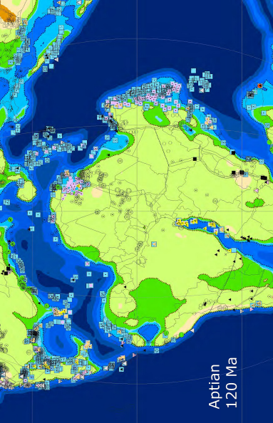
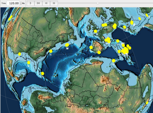
The results of all the machinations described above should be something that looks like Figure 9. This figure shows early Cretaceous coral reefs plotted on a map for the Aptian (120 Ma).

You can plot a numeric label or a symbol, but not both. If you want to plot a labels and a symbol, make two files – one with the numeric symbols and another with the labels (Figure 10).

I hope that these instructions worked for you. If not, feel free to contact me with comments or questions at: cscotese@gmail.com. The folks at EarthByte should also be able to help you with any questions about GPlates, but if your questions concern the symbol files or the PaleoData program, they will probably tell you to contact me, anyway!

References Cited

Baatsen, M., van Hinsbergen, D.J.J., von der Heydt, A.S., Dijkstra, H.A., Sluijs, A., Abels, H.A., and Bijl, P.K., 2015. A generalized approach for reconstructing geographical boundary conditions for palaeoclimate modeling, Climate of the Past Discussions, v. 11, p. 4917-4942.

Boucot, A.J., Chen Xu, and Scotese, C.R, 2013. Phanerozoic Paleoclimate: An Atlas of Lithologic Indicators of Climate, SEPM Concepts in Sedimentology and Paleontology, (Print-on Demand Version), No. 11, 478 pp., ISBN 978-1-56576-289-3, October 2013, Society for Sedimentary Geology, Tulsa, OK.

Haq, B. U., Hardenbol, J., and Vail, P.R., 1987. Chronology of Fluctuating Sea Levels Since the Triassic, Science, v. 235, p. 1156-1167.

Haq, B.U., and Schutter, S. R., 2009. A Chronology of Paleozoic Sea-Level Changes, Science, v. 322, p. 64-68.

Jakobsson, M., MacNab, R., Cherkis, N., and Schenke, H-W, 2004. The International Bathymetric Chart of the Arctic Ocean (IBCAO), Research Publication RP-2, National Geophysical Data Center, Boulder, CO.

Lythe, M.B., Vaughan, D.G., and the BEDMAP Consortium, 2000. BEDMAP: Bed Topography of the Antarctic, Misc. 9, scale 1:10,000,000, British Antarctic Survey, Cambridge, U.K. Miller, K.G., Kominz, M.A., Browning, J.V., Wright, J.D., Mountain, G.S., Katz, M.E., Sugarman, P.J., Cramer, B.S., Christie-Blick, N., and Pekar, S.F., 2005. The Phanerozoic Record of Global Sea Level Change, Science, v. 310, p. 1293-1298.

Moore, T.L., and C.R. Scotese, 2010. The Paleoclimate Atlas (ArcGIS), Geological Society of America, 2010 Annual Meeting, Abstracts with Programs, 42:598.

Ogg, J.G., Ogg, G, and Gradstein, F.M., 2008. The Concise Geologic Time Scale, Cambridge University Press, 177 pp.

Parsons, B. and Sclater, J.G., 1977, An analysis of the variation of ocean floor bathymetry and heat flow with age, Journal of Geophysical Research, v. 82, no. 5, p. 803-827. Peltier, W.R., 2004. Global Glacial Isostasy and the Surface of the Ice-Age Earth: The ICE-5G (VM2) Model and GRACE, Annual Review of Earth and Planetary Sciences, v. 32, p. 111-149. Rees, P.M., Ziegler, A.M., Gibbs, M.T., Kutzbach, J.E., Behling, P., and Rowley, D.B., 2002. Permian phytogeographic patterns and climate data/model comparisions, Journal of Geology, v. 110, p. 1-31.

Rees, P.M., Ziegler, A.M., and Valdes, P.J., 2000. Jurassic phytogeography and climates: new data and model comparisions, in B.T. Huber, K.G. Macleod, and S.L. Wing (editors), Warm Climates in Earth History, Cambridge University Press, p. 297-318.

Ross, C.A., and Ross, J.R.P., 1985. Late Paleozoic depositional Sequences are synchronous and worldwide, Geology, (March), v. 13, p. 194-197.

Rowley, D.B., and Currie, 2006. Paleo-altimetry of the late Eocene to Miocene Lunpola basin, central Tibet, Nature, v. 439, p. 677-681.

Rowley, D.B., and Garzione, C.N., 2007. Stable isotope-based paleoaltimetry, Annual Review of Earth and Planetary Science, v. 35, p. 463-508.

Rowley, D.B., Pierrehumbert, R.T., Currie, and Currie, B.S., 2001. A new approach to stable isotope-based paleoaltimetry: implications for paleoaltimetry and paleohypsometry of the

High Himalaya since the Late Miocene, Earth and Planetary Science Letters, v. 188, p.253- 268.

Scotese, C.R. and Sager, W.W., 1988. 8th Geodynamics Symposium, Mesozoic and Cenozoic Plate Reconstructions, Tectonophysics, v. 155, issues 1-4, p. 1-399

Scotese, C.R., Phanerozoic plate tectonic reconstructions Atlas Scotese, C.R., 1990. Atlas of Phanerozoic Plate Tectonic Reconstructions, PALEOMAP Progress 01-1090a, Department of Geology, University of Texas at Arlington, Texas, 57 pp.

Scotese, C.R., 2001. Animation of Plate Motions and Global Plate Boundary Evolution since the Late Precambrian, Geological Society of America, 2001 Annual Meeting, Boston, (November 2–6), Abstracts with Programs, v. 33, issue 6, p.85.

Scotese, C.R., 2002. 3D paleogeographic and plate tectonic reconstructions: The PALEOMAP Project is back in town, presented at Houston Geological Society International Exploration Dinner Meeting, Houston, TX, May 20, 2002, The Bulletin of the Houston Geological Society, v. 44, issue 9, p. 13-15

Scotese, C.R., 2008a, The PALEOMAP Project PaleoAtlas for ArcGIS, version 1, Volume 1, Cenozoic Paleogeographic, Paleoclimatic and Plate Tectonic Reconstructions, PALEOMAP Project, Arlington, Texas.

Scotese, C.R., 2008b, The PALEOMAP Project PaleoAtlas for ArcGIS, version 1, Volume 2, Cretaceous Paleogeographic, Paleoclimatic, and Plate Tectonic Reconstructions, PALEOMAP Project, Arlington, Texas.

Scotese, C.R., 2008c, The PALEOMAP Project PaleoAtlas for ArcGIS, version 1, Volume 3, Triassic and Jurassic Paleogeographic, Paleoclimatic, and Plate Tectonic Reconstructions, PALEOMAP Project, Arlington, Texas.

Scotese, C.R., 2008d, The PALEOMAP Project PaleoAtlas for ArcGIS, v.1, Volume 4, Late Paleozoic Paleogeographic, Paleoclimatic, and Plate Tectonic Reconstructions, PALEOMAP Project, Arlington, Texas.

Scotese, C.R., 2008e, The PALEOMAP Project PaleoAtlas for ArcGIS, v.1, Volume 5, Early Paleozoic Paleogeographic, Paleoclimatic, and Plate Tectonic Reconstructions, PALEOMAP Project, Arlington, Texas.

Scotese, C.R., 2008f, The PALEOMAP Project PaleoAtlas for ArcGIS, v.1, Volume 6, Late Precambrian Paleogeographic, Paleoclimatic, and Plate Tectonic Reconstructions, PALEOMAP Project, Arlington, Texas.

Scotese, C.R, 2014a. Atlas of Phanerozoic Oceanic Anoxia (Mollweide Projection), Volumes 1-6, PALEOMAP Project PaleoAtlas for ArcGIS, PALEOMAP Project, Evanston, IL. Scotese, C.R., 2014b. Atlas of Plate Tectonic Reconstructions (Mollweide Projection), Volumes 1-6, PALEOMAP Project PaleoAtlas for ArcGIS, PALEOMAP Project, Evanston, IL. Scotese, C.R., 2016. The PALEOMAP Global Plate Tectonic Model for GPlates, Earthbyte Publication (in prep.).

Scotese, C.R., Boucot, A.J, and Chen Xu, 2014. Atlas of Phanerozoic Climatic Zones (Mollweide Projection), Volumes 1-6, PALEOMAP Project PaleoAtlas for ArcGIS, PALEOMAP Project, Evanston, IL.

Scotese, C.R., Dammrose, R., 2008. Plate Boundary Evolution and Mantle Plume Eruptions during the last Billion Years, Geological Society of America 2008 Annual Meeting, October 5- 9, 2008, Houston, TX, Abstracts with Programs, v. 40, issue 6, Abstract 233-3, p. 328.

Scotese, C.R. and McKerrow, W.S., 1990. Revised world maps and introduction, in Paleozoic Paleogeography and Biogeography, W.S. McKerrow and C.R. Scotese (editors), Geological Society of London, Memoir 12, p. 1-21.

Scotese, C.R., and Moore, T.L., 2014a. Atlas of Phanerozoic Ocean Currents and Salinity (Mollweide Projection), Volumes 1-6, PALEOMAP Project PaleoAtlas for ArcGIS, PALEOMAP Project, Evanston, IL.

Scotese, C.R., and Moore, T.L., 2014b. Atlas of Phanerozoic Rainfall (Mollweide Projection), Volumes 1-6, PALEOMAP Project PaleoAtlas for ArcGIS, PALEOMAP Project, Evanston, IL. Scotese, C.R., and Moore, T.L., 2014c. Atlas of Phanerozoic Temperatures (Mollweide Projection), Volumes 1-6, PALEOMAP Project PaleoAtlas for ArcGIS, PALEOMAP Project, Evanston, IL.

Scotese, C.R., and Moore, T.L., 2014d. Atlas of Phanerozoic Winds and Atmospheric Pressure (Mollweide Projection), Volumes 1-6, PALEOMAP Project PaleoAtlas for ArcGIS, PALEOMAP Project, Evanston, IL.

Scotese, C.R., and Moore, T.L., 2014e. Atlas of Phanerozoic Upwelling Zones (Mollweide Projection), Volumes 1-6, PALEOMAP Project PaleoAtlas for ArcGIS, PALEOMAP Project, Evanston, IL.

Smith, W.H.F., and Sandwell, D.T., 1997. Global Sea Floor Topography from Satellite Altimetry and Ship Depth Soundings, Science, v. 277, p. 1956-1962.

Smith, William, 1815. A Delineation of the Strata of England and Wales and part of Scotland, Geological Society of London.

Stein, C.A. and Stein, S. 1992. A model for the global variation in oceanic depth and heat flow with lithospheric age, Nature, v. 359, p. 123-129.

Verard, C., Hochard, C., Baumgartner, P.O., and Stampfli, G.M., 2015. 3D palaeogeographic reconstructions of the Phanerozoic versus sea-level and Sr- ratio variations. Journal of Palaeogeography, vol. 4, no. 1, p. 64-84.

Ziegler, A.M., 1975. A Proposal to Produce an Atlas of Paleogeographic Maps, Department of Geophysical Sciences, University of Chicago, 17 pp.

Ziegler, A.M., and Scotese, 1977. Thoughts on Format for the Forthcoming “Atlas of Paleogeographic Maps”, Department of Geophysical Sciences, University of Chicago, 6 pp. Ziegler, A.M., Rowley, D.B., Lottes, A.L., Sahagian, D.L., Hulver, M.L., and Gierlowski, T.C., 1985. Paleogeographic interpretation: With an Example from the Mid-Cretaceous, Annual Review of Earth Sciences, volume 13, p. 385-425.

Appendix 1. Annotated Bibliography of Key Paleogeographic References

Explanation: Each bibliographic citation is followed by the region of the world, the number of maps, and the time intervals.

For example: Dercourt, J., Ricou, L.E., and Vrielynick, B., 1993. Atlas Tethys, Palaeoenvironmental Maps, Gauthier-Villars, Paris, 32 pp., / Tethys region from northern Australia to North America/ 14 maps / Permian (Late Murgabian), Triassic (Late Anisian, Late Norian), Jurassic (Middle Toarcian, Callovian, Early Kimmeridgian, Late Tithonian), Cretaceous (Early Aptian, Late Cenomanian, Late Maastrichtian), Tertiary (Lutetian, Late Rupelian, Late Burdigalian, Tortonian)/

References Cited in Table 4.

Blakey, R.C., 2002. Global Paleogeography, Rectilinear Projection, Colorado Plateau Geosystems, Inc., Flagstaff, AZ, (DVD)/Global/31 maps/ Middle Neoproterozoic (750Ma, 690Ma), Late Neoproterozoic (660Ma, 600Ma), latest Neoproterozoic (560Ma), Early Cambrian (540Ma), Late Cambrian (500Ma), Early Ordovician (480Ma), Middle Ordovician (470Ma), Late Ordovician (450Ma), latest Ordovician (440Ma), Early Silurian (430Ma), Early Devonian (400Ma), Middle Devonian (370Ma), Early Carboniferous (340Ma), Late Carboniferous (300Ma), Early Permian (280Ma), Late Permian (260Ma), Early Triassic (240Ma), Middle Triassic (220Ma), latest Triassic (200Ma), Middle-Late Jurassic (170Ma), Late Jurassic (150Ma), Aptian (120Ma), Albian (105Ma), Cenomanian-Turonian (90Ma), Maastrichtian (65Ma), Early Eocene (50Ma), Oligocene (35Ma), Early Miocene (20Ma), Modern (000Ma)/

Blakey, R.C., 2008. Gondwana paleogeography from assembly to breakup - A 500 m.y. odyssey, Geological Society of America Special Papers, v. 441, p. 1-28./Gondwana/ 18 maps/Late Cambrian (500Ma), Middle Ordovician (470Ma), Late Ordovician (450Ma), Silurian (430Ma), Early Devonian (400Ma), Mississippian (340Ma), Pennsylvanian (300Ma), Early Permian (280Ma), Middle Triassic (240Ma), Early Jurassic (200Ma), Middle Jurassic (170Ma), Late Jurassic (150Ma), Early Cretaceous (120Ma), mid Cretaceous (105Ma), Late Cretaceous (90Ma), Late Cretaceous (75Ma), Eocene, (50Ma), Oligocene (35Ma)/

Blakey, R.C., 2011. Paleogeography of Europe, Colorado Plateau Geosystems, Inc., Flagstaff, AZ, (DVD)/Western Europe/26 maps/Late Precambrian (600Ma, 575 Ma, 550Ma), Early Cambrian (525Ma), Late Cambrian (500Ma), Early Ordovician (475Ma), Late Ordovician (450Ma), Silurian (425 Ma), Early Devonian (400Ma), Late Devonian (375Ma), Early Mississippian (350Ma), Late Mississippian (325Ma), Late Pennsylvanian (300Ma), Early Permian (275 Ma), Early Triassic (250Ma), Late Triassic (225Ma), Early Jurassic (200Ma), Middle Jurassic (175Ma), Late Jurassic (150Ma), Early Cretaceous (125Ma), Late Cretaceous (100Ma, 75Ma), Early Eocene (50Ma), Late Oligocene (25Ma), Middle Miocene (13Ma), Present-day (0Ma)/

Blakey, R.C., 2013. Key Time Slices of North American Geologic History, Colorado Plateau Geosystems, Inc., Flagstaff, AZ, (DVD)/Western Europe/37 maps/Early Cambrian

(540Ma), Late Cambrian (500Ma), Early Ordovician (485Ma), Middle Ordovician (470Ma), Late Ordovician (450Ma), Late Silurian (420 Ma), Middle Devonian (390Ma), Late Devonian (375Ma), Late Devonian-Early Mississippian (360Ma), Early Mississippian (345Ma), Late Mississippian (325Ma), Early Pennsylvanian (315Ma), Middle Mississippian (308Ma), Late Pennsylvanian (300Ma), Early Permian (280 Ma), Middle Permian(260Ma), Early Triassic (245Ma), Late Triassic (220Ma), Early Jurassic (195Ma, 180Ma), Middle Jurassic (170Ma), Late Jurassic (150Ma), Early Cretaceous (130Ma, 115Ma, 105Ma), Late Cretaceous (92Ma, 85Ma, 72Ma), Paleocene(60Ma), Early Eocene (50Ma), Early Eocene-Late Oligocene (35Ma)Late Oligocene (25Ma), Early Miocene (20Ma), Late Miocene (10Ma), Pliocene (5 Ma), Pleistocene (20Ka),Present-day (0Ma)/

Boucot, A.J., Chen Xu, Scotese, C.R., and Fan Jun-Xuan, 2009. Atlas of Phanerozoic Lithologic Indicators of Climate, Science Press, Nanjing,204 pp. (in

Chinese)./Global/27 maps/ Early Cambrian (540Ma), Middle and Late Cambrian (520Ma), Early Ordovician(480Ma), Middle and Late Ordovician(440Ma), Silurian (420Ma), Early Devonian(400Ma), Middle Devonian(380Ma), Late Devonian(360Ma), Early Mississippian (340Ma), Late Mississippian (320Ma), Late Pennsylvanian (300Ma), latest Pennsylvanian-earliest Permian (295Ma), Early Permian (280Ma), Late Permian (260Ma), Early Triassic (240Ma), Middle Triassic (220Ma), Late Triassic (210Ma), Early and Middle Jurassic (180Ma), Late Jurassic (160Ma), Early Cretaceous (120Ma), early Late Cretaceous (100Ma), late Late Cretaceous (80Ma), Paleocene (60Ma), Early Eocene (50Ma), Middle and Late Eocene (40Ma), Oligocene (30Ma), Miocene (20Ma)/

Bozhko, N.A., and Khain, V.E., 1987. Gondwana Paleotectonic Maps, Ministry of Higher and Secondary Special education of the U.S.S.R., and Ministry of Geology, U.S.S.R., produced by the Geological Complex of Central Regions of the U.S.S.R., 30 pp. / Africa, South America, Arabia, Madagascar, India, Antarctica, Australia / 22 maps/ Katarchean (3500 my), Early Archean (3.5 by – 3.0 by), Late Archean (3.0 by – 2.6 by), Early Proterozoic (2.6 by – 1.9 by), Early Proterozoic (1.9 by – 1650 my), Early Riphean (1650 -1350 my), Middle Riphean (1350 – 1050 my), Late Riphean (1050 – 700 my), Vendian (700 – 570 my), Cambrian, Ordovician, Silurian, Devonian, Carboniferous, Permian, Triassic, Early-Middle Jurassic (180 my), Late Jurassic – Early Cretaceous (160 my), Late Cretaceous (65 my), Paleocene-Eocene (35 my), Oligocene-Miocene (5 my), Pliocene-Holocene/

Cook, P.J., 1990. Australia: Evolution of a Continent. Bureau of Mineral Resources (BMR), Paleogeographic Group, Australian Government Publishing Service, Canberra. / Australia / 69 maps/ Cambrian (5 maps), Ordovician (4 maps), Silurian (3 maps), Devonian (10 maps), Carboniferous (6 maps), Permian (7 maps), Triassic (6 maps), Jurassic (10 maps), Cretaceous (11 maps), Cenozoic (7 maps)/

Cook, T.D., and Bally, A.W.,1975. Stratigraphic Atlas of North America and Central America, Princeton University Press, Princeton, New Jersey, 272 pp. / North America / 42 maps/Cambrian (lower, middle, upper ), Ordovician (lower, middle, middle-upper, upper), Silurian (Medina, Clinton, Lockport, Salina), Devonian (lower, middle, Frasnian, Famennian), Mississippian (Pre-Chesterian, Chesterian), Pennsylvanian (Atokan-Morrowan, Desmoinesian, Missourian, Virgilian), Permian (Wolfcampian, Leonardian, Guadalupian, Ochoan), Triassic (lower, middle, upper), Jurassic (lower,

middle, Oxfordian, Portlandian-Kimmeridgian), Cretaceous (top Jurassic-mid Aptian, mid Aptian- mid Cenomanian, mid Cenomanian – top Turonian, Coniacian-Santonian, Campanian-Maestrichtian), Tertiary (Paleocene, Eocene, Oligocene, Miocene, Pliocene)/

Cocks, L.R.M., and Scotese, C.R., 1991. The Global Biogeography of the Silurian Period, in M.G. Bassett, P.D. Lane, and D. Edwards., The Murchison Symposium, Special Papers in Palaeontology, no. 44, Palaeontological Association, London, p. 109-122. /Global/3 maps/Silurian (Llandovery, Wenlock,), Devonian (Lochkovian)/

Cope, J.C. W., Ingham, J.K., and Rawson, P.F., 1992. Atlas of Paleogeography and Lithofacies, Geological Society of London, Memoir 13, 153 pp. / Great Britain and the North Sea/ ~80 maps/Upper Proterozoic (Stoer, Torridonian, Dalradian), Cambrian (Comley, St. David’s, Merioneth), Ordovician (Tremadoc, Arenig, Llanvirn, Llandeilo, Caradoc, Ashgill, Hirnantian), Silurian (latest Ashgill early Llandovery, early Llandovery, middle Llandovery, late Llandovery, early Wenlock, late Wenlock, early Ludlow, late Ludlow, early Ludfordian, late Ludfordian, earliest Pridoli, mid Pridoli), Devonian (Lochkovian, Pragian-Emsian boundary, Givetian, Frasnian-early Famennian), Carboniferous (Devonian-Carboniferous boundary, mid Courceyan, latest Courceyan- early Chadian, Arundian, Brigantian, early Namurian, late Namurian, Westphalian A, Westphalian D), Permian (Early Permian, Lower Zechstein 1, Upper Zechstein 1, Lower Zechstein 2, Upper Zechstein 2, Lower Zechstein 3, Upper Zechstein 3, Zechstein 4, Zechstein 5), Triassic (early to mid Scythian, Anisian to earliest Carnian, latest Norian to earliest Rhaetian, mid to late Rhaetian, Jurassic (Early Hettangian, Early Pliensbachian, Late Pliensbachian, Mid Toracian, Early Aalenian, Late Aalenian, Early Bajocian, Late Bajocian, Mid Bathonian, Late Bathonian, Early Callovian, Mid Callovian, Mid Oxfordian, Late Kimmeridgian, Portlandian), Cretaceous (Berriasian, Mid Hauterivian, Late Aptian, Latest Albian, Early Cenomanian, Late Campanian), Paleogene and Neogene (Paleocene, early Paleocene, Early Eocene, Mid Eoccene, Late Eocene, Mid-Late Oligocene, Miocene-Pliocene), Quaternary/

Copper, P. and Scotese, C.R., 2003. Megareefs in Mid-Devonian supergreenhouse climates. In, M.A. Chan & A.W. Archer (eds.), Extreme depositional environments: mega end members in geologic time, Geological Society America Special Paper 370 p. 209-230. /Global / 3 maps/ Devonian (Emsian, Givetian, Eifelian) /

Dercourt, J., Ricou, L.E., and Vrielynick, B., 1993. Atlas Tethys, Palaeoenvironmental Maps, Gauthier-Villars, 307 pp., Paris. / Tethys from northern Australia to eastern North America/ 14 maps/Permian (Late Murgabian), Triassic (Late Anisian, Late Norian), Jurassic (Middle Toarcian, Callovian, Early Kimmeridgian, Late Tithonian), Cretaceous (Early Aptian, Late Cenomanian, Late Maastrichtian), Tertiary (Lutetian, Late Rupelian, Late Burdigalian, Tortonian)/

Dercourt, J., Gaettani, M., Vrielynck, B., Barrier, E., Biju-Duval, Brunet, M.F., Cadet, J.P., Crasquin, S., and Sandulescu, M., 2000. Atlas Peri-Tethys, Paleogeographical Maps, Commission for the Geologic Map of the World (CCGM/CGMW, 24 maps and explanatory notes, 269 pp., Paris. / Western Tethys from Caspian Sea to Grand Banks/24 maps/ Pennsylvanian (Moscovian), Permian (Artinskian, Wordian), Triassic (Olenekian, Early Ladinian, Late Norian), Jurassic (Late Sinemurian, Middle Toarcian, Middle Callovian, Early Kimmeridgian, Early Tithonian), Cretaceous (Early Hauterivian, Early Aptian, Late Cenomanian, Early Campanian, Late Maastrichtian),

Paleogene (Early-Middle Ypresian, Late Lutetian, Late Rupelian), Neogene (Early Burdigalian, Early Langhian, Late Tortonian, Piacenzian/Gelasian. Last Glacial Maximum)

Evans, D., Graham, C., Armour, A., and Bathurst, P., 2003. The Millenium Atlas: Petroleum Geology of the Central and Northern North Sea, Geological Society of London, 389 pp. /Central North Sea/>46 maps/ Permian (Early-Middle, Late), Permo-Triassic, Triassic (Early TR00 Induan-Olenekian, early Middle TR10 Anisian-Ladinian, late Middle TR20 Carnian-Norian, Late TR30 TR40 TR50 Rhaetian-Sinemurian), Early and Middle Jurassic(early Pliensbachian, late Pliensbachian, early Torarcian-Aalenian, early Bajocian, late Bajocian, early Bathonian, early Callovian, middle-late Callovian), Late Jurassic (Callovian, early-late Oxfordian, late Oxfordian-early Kimmeridgian, early-late Kimmeridgian, late Kimmeridgian-early Volgian, early-middle Vogian, middle Volgian, middle Volgian-late Ryazanian), Early Cretaceous (late Ryazanian-early Valanginian, late Valanginian-late Barremian, early Aptian-early Albian), Late Cretaeous (Campanian-Maastrichtian), Paleocene (Maureen late Early Paleocene-early LatePaleocene, Lista Late Paleocene, Dornoch earliest Eocene, Balder early Eocene), Eocene( Early Eocene T66 T70, early middle Eocene T82, Middle Eocene T84 T92 T94 T96, Middle-Late Eocene T98), Oligocene-Holocene )(Rupelian CC4, Chattian CC5, Aquitanian-early Burdigalian CC5, late Burdigalian –early Serravalian CC6, middle Serravalian-Messinian CC7, Pliocene CC8)/

Golonka, J., Ross, M.I., and Scotese, C.R., 1994. Phanerozoic Paleogeographic and Paleoclimatic Modeling Maps, in A. F. Embry, B. Beauchamp, and D.J. Glass (editors), Pangea, Global Environments and Resources, Canadian Society of Petroleum Geologists, Memoir 17, p. 1-47. /Global/ 29 maps/Cambrian (Early & Late), Ordovician (Tremadocian, Llandeilo), Silurian (Llandovery, Wenlock), Devonian (Gedinnian, Givetian, Famennian), Carboniferous (Visean, Westphalian), Permian (Artinskian, Kazanian), Triassic (Induan, Norian), Jurassic (Pliensbachian, Callovian, Tithonian), Cretaceous (Valanginian, Aptian, Albian, Cenomanian, Coniacian, Maastrichtian), Tertiary (Thanetian, Lutetian, Chattian, Vindobonian, Present-day)/

Golonka, J., 2000. Cambrian-Neogene Plate Tectonic Maps, Rozprawy Habilitacyine No. 350, Wydawnictwo Uniwersytetu Jagiellonskiego, Krakow, 123 pp./Globa1/ 31 maps/ Cambrian(Early, Middle, latest Cambrian-early Ordovician), Ordovician(late Early early Middle,late Middle-Late), Silurian (Early, Late, latest Silurian-Early Devonian), Devonian (Early-Middle, Middle-Late, latest Devonian-Early Carboniferous), Carboniferous (Early,Late,latest Carboniferous-earliest Permian), Permian (Early, Late), Triassic (Early –earliest Late ,Late), Jurassic (Early-earliest Middle, Middle, latest Middle-Late), latest Jurassic – earliest Cretaceous, Cretaceous (Early, Early earliest Late, Late), Late Cretaceous-earliest Paleogene, Tertiary (Ypresian, Lutetian, Rupelian, Chattian-Aquitanian, Burdigalian-Serravallian, Tottonian-Gelasian)/

Hambrey, M.J., and Harland, W.B., 1981. Earth’s pre-Pleistocene glacial record, Cambridge University Press, Cambridge, 1004 pp. / Global/ >50 maps/pre-Pleistocene/ Hutchison, C.S., 1989. Geological Evolution of South-East Asia, Oxford University Press, Oxford, 368 pp./ Southeast Asia/8 maps/ Ordovician- Silurian, mid Silurian – mid Devonian, mid Devonian – Tournaisian, Visean – early Permian, mid Permian – Norian, Norian – late Jurassic, Late Jurassic – mid Cretaceous, mid Cretaceous – Neogene/

Hulver, M., 1985. Cretaceous Marine Paleogeography of Africa, Master’s Thesis, University of Chicago, Chicago, /Africa/5 maps/Cretaceous (Valanginian, Aptian, Cenomanian, Coniacian, Maastrichtian)/

Kazmin, V.G., and Natapov, L.M., 1998. The Paleogeographic Atlas of Northern Eurasia: Paleogeographic Maps on the Palinspastic Reconstruction (Orthographic Projection), Institute of Lithospheric Plates, Russian Academy of Natural Sciences, Moscow. /Northern Eurasia/26 maps/ 10 Ma (Serravalian & Tortonian), 20 Ma (Aquitanian, Burdigalian, & Langhian), 30 Ma (Oligocene), 40 Ma (Late Eocene), 50 Ma (Early & Middle Eocene), 60 Ma (Paleocene), 70 Ma (Maastrichtian), 80 Ma (Santonian & Campanian), 90 Ma (Cenomanian, Turonian, & Coniacian), 100Ma, (Late Albian), 110 Ma (Early Albian), 120 Ma (Aptian), 130Ma (Hauterivian & Barremian), 140 Ma (Berriasian & Valanginian), 150 Ma (Tithonian), 160 Ma (Callovian, Oxfordian, & Kimmeridgian), 180 Ma (Toarcian, Aalenian, Bajocian, and Bathonian), 195 Ma (Rhaetian, Hettangian, Sinemurian, & Pliensbachian), 210 Ma (Carnian & Norian), 240 Ma (Early – Middle Triassic), 255 (Late Permian – Zechstein), 280 Ma (Early Permian – Rotliegendes), 305 Ma (Pennsylvanian), 330 Ma (Early Carboniferous – Ivorian, Visean, & Serphukhovian), 355 Ma (Devono-Carbonifereous, Famennian & Hastarian), 380 Ma (Givetian & Frasnian)/

Khain, V.Ye., Ronov, A.B., and Balukhovsky, A.N., 1976. Cretaceous lithologic associations of the world, International Geology Review, v. 18, no.11, p. 1269-1295 (English translation from Russian) Sovetskaya Geologiya, 1976, v. 11, p. 10-39.

Khain, V.Ye., Ronov, A.B., and Balukhovsky, A.N., 1979. Paleogene lithologic associations of the continents, International Geology Review, v. 21, no.4, p. 415-446 (English translation from Russian) Sovetskaya Geologiya, 1976, v. 8, p. 10-45.

Khain, V.Ye., Ronov, A.B., and Balukhovsky, A.N., 1981. Neogene lithologic associations of the continents, International Geology Review, v. 21, no.4, p. 426-454 (English translation from Russian) Sovetskaya Geologiya, Sovetskaya Geologiya, 1976, v. 11, p. 3-35.

Khain, V.Ye., Ronov, A.B., and Seslavinsky, K.B., 1978. Silurian lithologic associations of the world, International Geology Review, v. 20, no.3, p. 249-268. (original Russian) Sovetskaya Geologiya, 1980, v. ??, no. 5?, p. 59-79.

Kriest, J., (1991), Plate-Tectonic Atlas, Exploration Bulletin, no. 258 (1995/5), Shell Exploration Company, Den Hague, 8 pp./Global/27 maps/ Early Cambrian (550Ma), Middle Cambrian (520Ma), Early Ordovician(490 Ma), Late Ordovician (460 Ma), Silurian (430Ma), Early Devonian (400Ma), Late Devonian (370Ma), Early Carboniferous (340Ma), Middle Carboniferous (310Ma), Permo-Carboniferous (290Ma), Early Permian (270Ma), Late Permian (250Ma), early Late Triassic (230Ma), Late Triassic (210Ma), Sinemurian/Pliensbachian (195Ma), Toarcian (180Ma), Bathonian (165Ma), Tithonian (150Ma), Hauterivian (135Ma), Aptian (120Ma), Albian (105Ma), Cenomanian/Turonian (90Ma), Campanian/Maastrichtian (75Ma), Selandian (60Ma), Lutetian (45Ma), Rupelian/Chattian (30Ma), Langhian (15Ma), Present-day (0Ma)/

Kiessling, W., 2001. Paleoclimatic significance of Phanerozoic Reefs, Geology, v. 29, no. 8, p. 751-754. / Phanerozoic Reef Paleolatitudes/

Kiessling, W., Flügel, and Golonka, J., 2002. Phanerozoic Reef Patterns, SEPM (Society for Sedimentary Geology) Special Publication Number 72, 775 pp. /Global/ >40 maps

/Cambrian (Early, Middle to early Late, Late Cambrian –Tremadocian), Ordovician (Tremadocian-early Darwillian, late Darwillian-Late Ordovician, Hirnantian), Silurian (Llandovery, Wenlock, Ludlow- early Pridoli), Devonian (Lochkovian-early Pragian, late Pragian-Emsian-Eifelian, Givetian, Frasnian, Famennian, Devono-Carboniferous Boundary), Carboniferous (Visean and Serpukhovian, Bashkirian-Kasimovian,Permo Carboniferous Boundary),Permian (middle, late), Triassic (Scythian-Carnian,Norian, Rhaetian), Jurassic (early, Bajocian and Bathonian, Callovian-lower Tithonian), Cretaceous (Berriasian,late Valangian-early Aptian,late Apian-middle Cenomanian, late Cenomanian-Santonian), Campanian-Danian, Tertiary (Thanetian Ypresian,Lutetian-Bartonian,Priabonian-Rupelian, Chattian-Aquitanian, Burdigalian Serravallian, Tortonian-Pliocene)/

Mallory, W.W., 1972. (editor), Geological Atlas of the Rocky Mountain Region, Rocky Mountain Association of Geologists, Denver, 331 pp. (available as pdf from AAPG)/Rocky Mountain States/ >62 maps/Cambrian (late early, early middle, late middle, middle Dresbach, late Dresbach, early Franconia, middle Franconia, middle Trempealeau, late Trempealeau), Ordovician (Canadian, lower Champlain, upper Champlain, lower Cincinnati, upper Cincinnati), Silurian (lower interlake, middle Interlake, upper Interlake), Devonian (Givetian, Frasnian, Famennian, uppermost Devonian-lowermost Mississippian), Mississippian (Kinderhook, Osage, Meramec, Chester), Pennsylvanian(Morrow, Atoka, DesMoines, Missouri, Virgil), Permian (lower Wolfcamp, upper Wolfcamp, lower Leonard, upper Leonard, Guadalup), Triassic (lower and middle?, late), Jurassic (Nugget, Piper, Nesson, Rierdon, Swift, Morrison), Cretaceous (Neocomian-Aptian, early Albian, middle-late Albian, late Skull Creek, latest Albian, early Belle Fourche, middle Greenhorn, middle Carlisle, early Niobrara, middle Niobrara, Telegraph Creek, latest Eagle, early Claggett, middle Judith River, middle Bearpaw, early Fox Hills, latest Cretaceous), Cenozoic (early Paleocene, late Paleocene, late-middle Eocene, late Eocene, Oligocene, Miocene, Pliocene, Quaternary)/

McKerrow, W.S., Dewey, J.F., and Scotese, C.R., 1991. The Ordovician and Silurian Development of the Iapetus Ocean, in M.G. Bassett, P.D. Lane, and D. Edwards (editors), The Murchison Symposium, Special Papers in Palaeontology, no. 44, Palaeontological Association, London, p. 165-178. /Circum-Iapetus Ocean/6 maps/Ordovician (Tremadoc, Arenig, Caradoc), Silurian (Llandovery, Ludlow), Devonian (Emsian)/

Moore, T.L., and C.R. Scotese., 2012, Ancient Earth: Breakup of Pangea, Vers. 1.0, iOS Mobile Application, retrieved from http://itunes.apple.com/ Global/24 maps/Modern (0 Ma), Last Glacial Maximum (20 ka), Messinian (6.3Ma), Middle/Late Miocene (10.5Ma), Early Miocene (19.5Ma), Early Oligocene (31.1 Ma), late Middle Eocene (38.8 Ma), Early Eocene (52.2Ma), PETM (55.8 Ma), Paleocene (60.6), KT Boundary (65.5Ma), Maastrichtian (68Ma), Early Campanian (80.3 Ma), Turonian (91.1Ma), late Albian (101.8Ma), early Albian (110.0Ma), early Aptian (121.8Ma), Hauterivian (132.0Ma), Berriasian (143.0Ma), latest Jurassic (148.2), Late Jurassic (158.4), Middle Jurassic (169.7Ma), Early Jurassic (179.3Ma), latest Triassic (201.6Ma)/

Moore, T.L., and C.R. Scotese., 2013, Ancient Earth: Assembly of Pangea, Vers. 1.0, iOS Mobile Application, retrieved from http://itunes.apple.com / Global/ 23 maps/latest Triassic (201.6Ma), late Late Triassic (210.0Ma), early Late Triassic (222.6), late

Middle Triassic (232.9Ma), early Middle Triassic (241.5Ma), Permo-Triassic Boundary (251.0Ma), late Middle Permian (263.1Ma), Middle Permian (268.2Ma), late Early Permian (280.0Ma), Early Permian (289.5Ma), latest Pennsylvanian (301.2Ma), late Mississippian (323.2Ma), middle Mississippian (341.1Ma), Late Devonian (379.9Ma), late Early Devonian (402.3Ma), latest Silurian (419.5Ma), Early Silurian (432.1Ma), latest Ordovician (444.7Ma), Middle Ordovician (464.5Ma), Early Ordovician (480Ma), Late Cambrian (494Ma), Middle Cambrian(520Ma), Cambrian-Precambrian Boundary (542Ma)/

Mossop, G. and Shetson, I., 1994. Geological Atlas of Western Canada Sedimentary Basins, Canadian Society of Petroleum Geologists, Calgary, 510 pp. /Western Canada/ >52 maps/ Cambrian (middle, late Cambrian-early Ordovician), Ordovician (latest early – early middle, earliest late, early late, late), Silurian (early, late Silurian – early Devonian), Devonian (early, early middle, early Givetian, middle Givetian, Givetian Frasnian, early Frasnian, middle Frasnian, late Frasnian, Famennian), Carboniferous (late Devonian –early Torunaisian, Late Tournaisian-early Visean, middle Visean Serpukhovian, Bashkirian-Moscovian), Permian (Asselian-Sakmarian, Artinskian, Roadian-Wordian), Triassic (early Triassic, Anisian-Ladinian, early middle Carnian, late Carnian-Norian), Jurassic (Sinemurian, Toarcian, early Bajocian, Bajocian, Bathonian-Callovian, late Oxfordian – middle late Tithonian), Cretaceous (latest Jurassic – earliest Cretaceous, Berriasian, Berriasian-Valanginian, latest Barremian – early late Aptian, late Aptian, earliest Albian, early Albian, late early Albian, middle Albian, Cenomanian, Turonian, early Campanian, late early Campanian, middle Campanian, late Campanian, middle Maastrichtian), Tertiary (earliest Paleocene, late early Paleocene – early late Paleocene)/

Pindell, J.L., Higgs, R., and Dewey, J.F., 1998. Cenozoic palinspastic reconstruction, paleogeographic evolution, and hydrocarbon setting of the northern margin of South America, in J.L. Pindell and C.L. Drake (eds.), Paleogeographic Evolution and Non Glacial Eustasy, Northern South America, Society for Sedimentary Geology (SEPM), Special Publication 58, p. 45-86. / northernmost South America/7 maps/Early Paleocene, Early Eocene, early Middle Eocene, early Late Eocene, Late Oligocene, late Early Miocene, late Middle Miocene/

Ronov, A.B., and Khain, V.Ye.,1954. Devonian lithologic formations (associations) of the world, Sovetskaya Geologiya v.41, p. 46-76. (in Russian)

Ronov, A.B., and Khain, V.Ye.,1955. Carboniferous lithologic formations (associations) of the world, Sovetskaya Geologiya v.48, p. 92-117. (in Russian)

Ronov, A.B., and Khain, V.Ye.,1956. Permian lithologic formations (associations)of the world, Sovetskaya Geologiya v.54, p. 20-36. (in Russian)

Ronov, A.B., and Khain, V.Ye.,1961. Triassic lithologic formations (associations) of the world, Sovetskaya Geologiya v.1, p. 27-48. (English translation from Russian, p. 73 - 103)

Ronov, A.B., and Khain, V.Ye.,1962. Jurassic lithologic formations (associations) of the world, Sovetskaya Geologiya v. 1, p. 3-34. (English translation from Russian, p. 7 - 29) Ronov, A.B., Khain. V. Ye., and Seslavinsky, K.B., 1982a, Upper Riphean lithologic complexes of the world, International Geology Review, v. 24, no. 9, p. 993-1008.

Ronov, A.B., Khain. V. Ye., and Seslavinsky, K.B., 1982b, Lower and middle Riphean lithologic complexes of the world, International Geology Review, v. 24, no. 5, p. 509- 525.

Ronov, A.B., Seslavinsky, K.B., and Khain, V. Ye., 1980. Vendian lithologic formations (associations) of the world, Sovetskaya Geologiya, v. ?, no.5, p. 37-59. (in Russian), translation in, International Geology Review, v. 14, no. 4, p. 373-394.

Ronov, A.B., Seslavinsky, K.B., and Khain, V. Ye., 1977. Cambrian lithologic formations (associations) of the world, Sovetskaya Geologiya, v. ??, no.12, p. 10-34. (in Russian), translation in, International Geology Review, v. 14, no. 4, p. 373-394.

Ronov, A.B., Khain. V. Ye., and Seslavinsky, K.B., 1976, Ordovician lithologic associations of the world, International Geology Review, v. 18, no. 12, p. 1395-1412. (original Russian) Sovetskaya Geologiya, 1976, v. ??, no.1, p. 7-27.

Ronov, A.B., Khain, V. Ye., and Balukhovsky, A., 1989. Atlas of Lithological Paleogeographical Maps of the World, Mesozoic and Cenozoic of the Continents, USSR Academy of Sciences,USSR State Committee for Public Education, Ministry of Geology of the USSR, 79 pp., Leningrad./Global/13 maps/Early Triassic, Middle Triassic, Late Triassic, Early Jurassic, Middle Jurassic, Late Jurassic, Early Cretaceous, Late Cretaceous, Paleocene, Eocene, Oligocene, Miocene, Pliocene/

Ronov, A.B., Khain, V. Ye., and Seslavinsky, K.B., 1984. Atlas of Lithological Paleogeographical Maps of the World, Late Precambrian and Paleozoic of the Continents, USSR Academy of Sciences, Ministry of Higher and Secondary Special Education of the USSR, Ministry of Geology of the USSR, 70 pp., Leningrad. / Global/ 18 maps/Early and Middle Riphean, Late Riphean, Vendian, Early Cambrian, Middle Cambrian, Late Cambrian, Early Ordovician, Middle Ordovician, Late Ordovician, Early Silurian, Late Silurian, Early Devonian, Middle Devonian, Late Devonian, Early Carboniferous, middle and Late Carboniferous, Early Permian, Late Permian/

Rowley, D.B., Raymond, A., Parrish, J.T., Lottes, A.L., Scotese, C.R., and Ziegler, A.M., 1985. Carboniferous paleogeographic, Phytogeographic, and paleoclimatic reconstructions, Internation Journal of Coal Geology, v. 5, p. 7-42./Global/2 maps/ Carboniferous (Visean, Westphalian)/

Schandelmeier, H., and Reynolds, P.O., 1997. Paleogeographic-Palaeotectonic Atlas of North-Eastern Africa, Arabia, and Adjacent Areas: Late Proterozoic to Holocene, A.A. Balkema, Rotterdam, 160 pp./Northeast Africa and Arabia/17 maps/Late Neoproterozoic (Vendian), Ordovician (Ashgill), Silurian (Llandovery), Devonian (Lochkovian), Carboniferous (lateTournaisian-early Visean, Bashkirian), Permian (Capitanian-Longtanian), Triassic (Norian), Jurassic (Toarcian, Kimmeridgian), Cretaceous (Valanginian, Aptian, Campanian-Maastrichtian), Tertiary (Lutetian, Chattian, Langhian, Quaternary-Holocene)/

Scotese, C.R., 1998, Digital Paleogeographic Map Archive on CD-ROM, PALEOMAP Project, Arlington, Texas./global/40 maps/ Middle Neoproterozoic (750Ma), Middle Neoproterozoic (720Ma), Middle Neoproterozoic (690Ma), Late Neoproterozoic (660Ma), Late Neoproterozoic (630Ma,) Late Neoproterozoic (600Ma), latest Neoproterozoic (560Ma), Early Cambrian (540Ma), Middle Cambrian (520Ma), Late Cambrian (500Ma), Early Ordovician (480Ma), Middle Ordovician (460Ma), Late Ordovician (440Ma), Early Silurian (430Ma), Middle-Late Silurian (420Ma), Early Devonian (400Ma), Middle Devonian (380Ma), Late Devonian (360Ma), Early

Carboniferous (340Ma), mid Carboniferous (320Ma), Late Carboniferous (300Ma), Early Permian (280Ma), Late Permian (260Ma), Early Triassic (240Ma), Middle Triassic (220Ma), Early Jurassic (180Ma), Middle-Late Jurassic (160Ma), Berriasian Barremian (140Ma), Aptian (120Ma), Albian (100Ma), Cenomanian-Turonian (90Ma), early Campanian (80Ma), Maastrichtian (70Ma), Paleocene (60Ma), Early Eocene (50Ma), Middle Eocene (40Ma), Oligocene (30Ma), Early Miocene (20Ma), Late Miocene (10Ma), Modern (000Ma)/

Scotese, C.R., 2001. Atlas of Earth History, Volume 1, Paleogeography, PALEOMAP Project, Arlington, Texas, 52 pp./Global/16 maps/Late Proterozoic-650Ma, Late Cambrian, Middle Ordovician, Middle Silurian, Early Devonian, Early Carboniferous, Late Carboniferous, Late Permian, Early Triassic, Early Jurassic, Late Jurassic, Late Cretaceous, KT Boundary, Middle Eocene, Middle Miocene, Pleistocene, Future +50Ma, Future +150Ma, Future +250Ma/

Scotese, C.R., 2004, Cenozoic and Mesozoic Paleogeography: Changing Terrestrial Biogeographic Pathways, in Frontiers of Biogeography: New Directions in the Geography of Nature, M.V. Lomolino and L.R. Heaney, (editors), Sinauer Associates, Inc., Sunderland, Massachusetts, p. 1-26./Global/18 maps/Triassic(Induan-Olenekian, Carnian-Norian), Jurassic(Hettangian-Sinemurian, Toarcian-Aalenian, Callovian Oxfodian), Cretaceous(Berriasian, Barremian-Aptian, Albian-Cenomanian, Turonian, Campanian, middle Maastrichtian), Tertiary(Selandian, Ypresian, Bartonian, Rupelian, Aquitainian-Burdigalian, Tortonian), Holocene/

Scotese, C.R., 2008a, The PALEOMAP Project PaleoAtlas for ArcGIS, version 1, Volume 1, Cenozoic Paleogeographic, Paleoclimatic and Plate Tectonic Reconstructions, PALEOMAP Project, Arlington, Texas. /Global/15 maps/ see Table 1/

Scotese, C.R., 2008d, The PALEOMAP Project PaleoAtlas for ArcGIS, v.1, Volume 4, Late Paleozoic Paleogeographic, Paleoclimatic, and Plate Tectonic Reconstructions, PALEOMAP Project, Arlington, Texas. /Global/24 maps/ see Table 1/

Scotese, C.R., 2014a. Atlas of Neogene Paleogeographic Maps (Mollweide Projection), Maps 1-7, Volume 1, The Cenozoic, PALEOMAP Atlas for ArcGIS, PALEOMAP Project, Evanston, IL. ResearchGate Academia. /Global/ 10 maps/ Map 01 Modern World (Holocene, 0.0 Ma) Transgressive Systems Tract, Map 02 Last Glacial Maximum (Pleistocene, 21,000 years ago) Anthropocene Supersequence Boundary, Map 03 Plio Pleistocene, (Gelasian & Piacenzian, 2.588 Ma Ma) Lowstand Systems Tract, Map 04 Latest Miocene (Messinian Event, 6.3 Ma) Maximum Flooding Surface, Map 05

Middle/Late Miocene, (Serravallian and Tortonian, 10.5 Ma) Messinian Supersequence Boundary & Tortonian Maximum Flooding Surface, Map 06 Middle Miocene (Langhian, 14.9 Ma) Maximum Flooding Surface, Map 07 Early Miocene (Aquitanian & Burdigalian, 19.5 Ma) Serravallian Supersequence Boundary, Aquitanian Maximum Flooding Surface/

Scotese, C.R., 2014b. Atlas of Paleogene Paleogeographic Maps (Mollweide Projection), Maps 8-15, Volume 1, The Cenozoic, PALEOMAP Atlas for ArcGIS, PALEOMAP Project, Evanston, IL. ResearchGate Academia, /Global/ 12 maps/ Map 08 Late Oligocene (Chattian, 25.7 Ma Ma) Aquitanian Superseqeunce Boundary & Late Oligocene Transgressive Systems Tract, Map 09 Early Oligocene (Rupelian, 31.1 Ma) Maximum Flooding Surface, Map 10 Late Eocene, (Priabonian, 35.6 Ma) Rupelian Supersequence Boundary & Priabonian Transgressive Systems Tract, Map 11 late Middle Eocene (Bartonian, 38.8 Ma) Bartonian Transgressive Systems Tract, Map 12 early Middle Eocene, (middle Lutetian, 44.6 Ma) Lutetian Maximum Flooding Surface & Lutetian Supersequence Boundary, Map 13 Early Eocene (Ypresian, 52.2 Ma) Ypresian Maximum Flooding Surface, Map 14 Paleocene/Eocene Boundary (PETM, Thanetian/Ypresian Boundary, 55.8 Ma) PETM Transgressive Systems Tract, Map 15 Paleocene (Danian & Thanetian, 60.6 Ma) Paleocene Maximum Flooding Surface & Danian Supersequence Boundary/

Scotese, C.R., 2014c. Atlas of Late Cretaceous Paleogeographic Maps, PALEOMAP Atlas for ArcGIS, volume 2, The Cretaceous, Maps 16 - 22, Mollweide Projection, PALEOMAP Project, Evanston, IL. ResearchGate Academia, /Global/ 7 maps/ Map 16 K/T Boundary (latest Maastrichtian, 65.5 Ma), Map 17 Late Cretaceous (Maastrichtian, 68 Ma), Map 18 Late Cretaceous (Late Campanian, 73.8 Ma), Map 19 Late Cretaceous (Early Campanian, 80.3 Ma), Map 20 Late Cretaceous (Santonian & Coniacian, 86 Ma), Map 21 Mid Cretaceous (Turonian, 91.1 Ma), Map 22 Mid Cretaceous (Cenomanian, 96.6 Ma)/

Scotese, C.R., 2014d. Atlas of Early Cretaceous Paleogeographic Maps, PALEOMAP Atlas for ArcGIS, volume 2, The Cretaceous, Maps 23-31, Mollweide Projection, PALEOMAP Project, Evanston, IL. ResearchGate Academia, /Global/ 14 maps/ Map 23 Early Cretaceous (late Albian, 101.8 Ma), Map 24 Early Cretaceous (middle Albian, 106 Ma), Map 25 Early Cretaceous (early Albian, 110 Ma) Albian Supersequence Boundary and Transgressive System Tract, Map 26 Early Cretaceous (late Aptian, 115.2 Ma), Map 27 Early Cretaceous (early Aptian, 121.8 Ma), Map 28 Early Cretaceous (Barremian, 127.5 Ma), Map 29 Early Cretaceous (Hauterivian, 132 Ma), Map 30 Early Cretaceous (Valanginian, 137 Ma) Barremian-Hauterivian Supersequence boundary and Transgressive Systems Tract, Map 31 Early Cretaceous (Berriasian, 143 Ma) Berriasian Supersequence boundary and Maximum Flooding Surface/

Scotese, C.R., 2014e. Atlas of Jurassic Paleogeographic Maps, PALEOMAP Atlas for ArcGIS, volume 3, The Jurassic and Triassic, Maps 32-42, Mollweide Projection, PALEOMAP Project, Evanston, IL. ResearchGate Academia, /Global/ 16 maps/ Map 32 Jurassic/Cretaceous Boundary (145.5 Ma) Berriasian Supersequence Boundary, Map 33 Late Jurassic (Tithonian, 148.2 Ma) Highstand Systems Track , Map 34 Late Jurassic (Kimmeridgian, 153.2) Maximum Flooding Surface, Map 35 Late Jurassic (Oxfordian, 158.4) Transgressive Systems Track, Map 36 Middle Jurassic (Callovian, 164.5 Ma) Transgressive Systems Tract, Map 37 Middle Jurassic (Bajocian &

Bathonian, 169.7 Ma) Kimmeridgian-Oxfordian Supersequence Boundary & Maximum Flooding Surface, Map 38 Middle Jurassic (Aalenian, 173.2 Ma) Bathonian-Bajocian Supersequence Boundary, Map 39 Early Jurassic (Toarcian, 179.3 Ma) Toarcian Supersequence Boundary and Maximum Flooding Surface, Map 40 Early Jurassic (Pliensbachian, 186.3 Ma) Maximum Flooding Surface, Map 41 Early Jurassic (Sinemurian, 193 Ma) Transgressive Systems Track, Map 42 Early Jurassic (Hettangian, 198 Ma) Pliensbachian Supersequence Boundary/

Scotese, C.R., 2014f. Atlas of Middle & Late Permian and Triassic Paleogeographic Maps, maps 43 - 48 from Volume 3 of the PALEOMAP Atlas for ArcGIS (Jurassic and Triassic) and maps 49 – 52 from Volume 4 of the PALEOMAP PaleoAtlas for ArcGIS (Late Paleozoic), Mollweide Projection, PALEOMAP Project, Evanston, IL. ResearchGate Academia, /Global/ 12 maps/ Map 43 Late Triassic (Rhaetian, 201.6 Ma) Lowstand Systems Tract, Map 44 Late Triassic (Norian, 210 Ma) Maximum Flooding Surface, Map 45 Late Triassic (Carnian, 222.6 Ma) Transgressive Systems Tract, Map 46 Middle Triassic (Ladinian, 232.9 Ma) Transgressive Systems Tract, Map 47 Middle Triassic (Anisian, 241.5 Ma) Lowstand Systems Tract, Map 48 Early Triassic (Induan & Olenekian, 248.5 Ma) Lowstand Systems Track, Map 49 Permo-Triassic Boundary (251 Ma) Norian Supersequence Boundary, Map 50 Late Permian (Lopingian, 255.7 Ma) Transgressive Systems Tract, Map 51 late Middle Permian (Capitanian, 263.1 Ma) Lowstand Systems Tract, Map 52 Middle Permian (Roadian & Wordian, 268.2 Ma) Maximum Flooding Surface/

Scotese, C.R., 2014g. Atlas of Permo-Carboniferous Paleogeographic Maps (Mollweide Projection), Maps 53 – 64, Volume 4, The Late Paleozoic, PALEOMAP Atlas for ArcGIS, PALEOMAP Project, Evanston, IL. ResearchGate, /Global/ 15 maps/ Map 53 Early Permian (Kungurian, 273.1 Ma) Highstand Systems Tract , Map 54 Early Permian (Artinskian, 280 Ma) Maximum Flooding Surface, Map 55 Early Permian (Sakmarian, 289.5 Ma) Maximum Flooding Surface, Map 56 Early Permian (Asselian, 296.8 Ma) Sakmarian Supersequence Boundary & Maximum Flooding Surface, Map 57 Late Pennsylvanian (Gzhelian, 301.2 Ma) Asselian Supersequence Boundary & Maximum Flooding Surface, Map 58 Late Pennsylvanian (Kasimovian, 305.3 Ma) Maximum Flooding Surface, Map 59 Middle Pennsylvanian (Moscovian, 309.5) Transgressive Systems Tract, Map 60 Early Pennsylvanian (Bashkirian, 314.9 Ma) Bashkirian Supersequence Boundary & Maximum Flooding Surface, Map 61 Late Mississippian (Serpukhovian, 323.2 Ma) Maximum Flooding Surface, Map 62 Middle Mississippian (late Visean, 332.5 Ma) Highstand Systems Tract, Map 63 Middle Mississippian (early Visean, 341.1 Ma) Maximum Flooding Surface, Map 64 Early Mississippian (Tournasian, 352.3 Ma) Maximum Flooding Surface/

Scotese, C.R., 2014h. Atlas of Devonian Paleogeographic Maps, PALEOMAP Atlas for ArcGIS, volume 4, The Late Paleozoic, Maps 65-72, Mollweide Projection, PALEOMAP Project, Evanston, IL. ResearchGate, /Global/ 8 maps/ Map 65 Devono-Carboniferous Boundary (359.2 Ma) Transgressive Systems Track, Map 66 Late Devonian (early Famennian, 370.3 Ma) Tournasian Supersequence Boundary, Map 67 Late Devonian (Frasnian, 379.9 Ma) Maximum Flooding Surface, Map 68 Middle Devonian (Givetian,388.2 Ma) Frasnian Supersequence Boundary, Map 69 Middle Devonian (Eifelian, 394.3 Ma) Transgressive Systems Tract, Map 70 Early Devonian (Emsian, 402.3 Ma) Maximum Flooding Surface, Map 71 Early Devonian (Pragian, 409.1 Ma)

Emsian Supersequence Boundary, Map 72 Early Devonian (Lochkovian, 413.6 Ma) Lochkovian Supersequence Boundary/

Scotese, C.R., 2014i. Atlas of Silurian and Middle-Late Ordovician Paleogeographic Maps (Mollweide Projection), Maps 73 – 80, Volumes 5, The Early Paleozoic, PALEOMAP Atlas for ArcGIS, PALEOMAP Project, Evanston, IL. ResearchGate, /Global/8 maps/

Map 73 Late Silurian (Ludlow & Pridoli, 419.5 Ma) Lochkovian Supersequence Boundary , Map 74 Middle Silurian (Wenlock, 425.6 Ma) Highstand System Tract , Map 75 Early Silurian (late Llandovery, 432.1 Ma) Maximum Flooding Surface, Map 76 Early Silurian (early Llandovery, 439.8 Ma) Transgressive Systems Tract, Map 77 Late Ordovician (Hirnantian, 444.7 Ma) Llandoverian Supersequence Boundary, Map 78 Late Ordovician (Ashgill, 448.3 Ma) Lowstand Systems Tract & Maximum Flooding Surface, Map 79 Late Ordovician (Caradoc, 456 Ma) Maximum Flooding Surface, Map 80 Middle Ordovician (Darwillian, 464.5 Ma) Llandeilian Supersequence Boundary/

Scotese, C.R., 2014j. Atlas of Cambrian and Early Ordovician Paleogeographic Maps (Mollweide Projection), Maps 81-88, Volumes 5, The Early Paleozoic, PALEOMAP Atlas for ArcGIS, PALEOMAP Project, Evanston, IL. ResearchGate, /Global/ 8 maps/ Map 81 Early Ordovician (Arenig, 472.4 Ma) Arenigian Supersequence Boundary , Map 82 Early Ordovician (Tremadoc, 480 Ma) Maximum Flooding Surface , Map 83 Cambro Ordovician Boundary (488.3 Ma) Tremadocian Supersequence Boundary, Map 84 Late Cambrian (Furongian, 494 Ma) Croixian Supersequence Boundary, Map 85 early Late Cambrian (510 Ma) Transgressive Systems Tract, Map 86 Middle Cambrian (520 Ma) Transgressive Systems Tract, Map 87 Early Cambrian (531.5 Ma) Albertan Supersequence Boundary, Map 88 Cambrian-Precambrian Boundary (542 Ma) Caerfaian Supersequence Boundary/

Scotese, C.R., Bambach, R.J., Barton, C., Van der Voo, R., and Ziegler, A.M., 1979. Paleozoic Basemaps, Journal of Geology, v.87, no. 3, p. 217-277. /Global/ 7 maps/Cambrian(late Franconian), Ordovician (Llandeilo-earliest Caradoc), Silurian (Wenlock), Devonian (Emsian), Carboniferous (Visean, Westphalian), Permian (Kazanian)/

Scotese, C.R., and Golonka J. 1992. Paleogeographic Atlas, PALEOMAP Progress Report 20-0692, Department of Geology, University of Texas at Arlington, Texas, 34 p. /Global/ 28 maps/Cambrian (Early & Late), Ordovician (Tremadocian, Llandeilo), Silurian (Llandovery, Wenlock), Devonian (Gedinnian, Givetian, Famennian), Carboniferous (Visean, Westphalian), Permian (Artinskian, Kazanian), Triassic (Induan, Norian), Jurassic (Pliensbachian, Callovian, Tithonian), Cretaceous (Valanginian, Aptian, Cenomanian, Coniacian, Maastrichtian), Tertiary (Thanetian, Lutetian, Chattian, Vindobonian, Present-day)/

Scotese, C.R., and Langford, R.P., 1995. Pangea and the Paleogeography of the Permian, in The Permian of Northern Pangea, volume 1, Paleogeography, Paleoclimates, Stratigraphy, P.A. Scholle, T.M. Peryt, and D.S. Ulmer-Scholle (editors), Sproinger Verlaf, Berlin, p.3-19. / Global/ 2 maps/ Permian (late Asselian-mid Sakmarian, Kazanian)/

Scotese, C.R., and Winn, K., 1987. Phanerozoic Paleogeographic Maps, Paleoceanographic Mapping Project (POMP) Progress Report 33-1287, 31 pp. (UTIG Technical Report 84)/ Global / 14 maps/ Cambrian(late-Franconian), Ordovician (Llandeilo-Caradoc), Silurian (Wenlock), Devonian (Emsian), Carboniferous (Visean, Westphalian), Permian (Kazanian), Triassic (Induan), Jurassic (Pliensbachian, Volgian), Cretaceous

(Cenomanian, Maastrichtian), Tertiary (Lutetian, Vindobonian)/

Smith, A.G., Smith, D.G., and Funnell, B.M., 1994. Atlas of Mesozoic and Cenozoic Coastlines, Cambridge University Press, 99 pp., /Global/31 maps/Triassic (Scythian, Ladinian-Anisian, Rhaetian-Norian-Carnian), Jurassic (Hettangian, Sinemurian, Pliensbachian, Toarcian, Bajocian, Callovian, Oxfordian, Kimmeridgian, Tithonian), Cretaceous (Valanginian-Berriasian, Barremian-Hauerivian, Aptian, Albian, Cenomanian, Turonian, Coniacian, Santonian, Campanian, Maastrichtian), Tertiary (Thanetian-Danian, Ypresian, Bartonian-Lutetian, Priabonian, Oligocene, Burdigalian Aquitainian,Serravallian-Langhian,Messinian-Tortonian,Pliocene)/

Ulmishek, G.F., and Klemme, H.D., 1990. Depositional Controls, Distribution, and Efffectiveness of the World’s Petroleum Source Rocks, U.S.G.S. Bulletin 1931, Denver, 59 pp./Global/ 6 maps/Silurian, Upper Devonian-Tournaisian, Pennsylvanian-Lower Permian, Upper Jurassic, Middle Cretaceous, Oligocene-Miocene/

Veevers, J.J. 1984. Phanerozoic Earth History of Australia, Oxford Monographs on Geology and Geophysics, no. 2, Oxford University Press, New York, 418 pp. / Australia/ 44 maps/Precambrian (1000 Ma, Adelaidean – 850 to 650 Ma, Ediacaran), Cambrian (Early, Middle, late Early, Late), Ordovician (early,late Early,Middle, Late), Silurian(Early, mid, Late), Siluro-Devonian,Devonian(Early, late Early, early Middle, late Middle, early Late,latest), latest Devonian-earliest Carboniferous, Carboniferous (mid), Permo-Carboniferous Boundary, Permo-Triassic Boundary, Triassic (Scythian, late), Jurassic (Middle, Late), Cretaceous (earliest, early, Aptian, Aptian-Albian, Albian, Cenomanian, Turonian, Campanian, Maastrichtian), Tertiary (Paleocene, Eocene (middle – late), latest Eocene, Eocene-Oligocene, Miocene,Modern) /

Veevers, J.J., and Powell, C. McA., 1994. Permian-Triassic Pangean Basins and Foldbelts along the Panthalassan Margin of Gondwanaland, Geological Society of America, Memoir 184, 368 pp., Boulder, Colorado. /Australia, South Africa, Southern South America, Antarctica/41 maps`/ Permian(late Early, Early-Middle,Late), Permo Triassic Boundary, Triassic(Early, early Middle,Middle,late Middle, Late), Jurassic/ South Africa/ uppermost Table Mountain (Pragian-Emsian), Bokkeveld (Emsian and Givetian/Fasnian), Witteberg(Late Devonian), Dwyka (latest Carboniferous-earliest Permian), lower & middle Ecca(Early, Middle), Upper Ecca (Late Permian), Beaufort (Late Permian- Early Triassic), Molteno(Late Triassic), Karro volcanics (latest Triassic-Early Jurassic)/ Southern South America/Cambrian, Ordovician, Silurian, Early-Middle Devonian, Early-mid Carboniferous, Early Carboniferous-basal Permian, Late Carboniferous-Early Permian,Late Carboniferous-Late Permian, Early Permian Early Triassic/Synthesis/latest Devonian, Early-Middle Permian, Late Permian, Permo-Triassic, early Triassic, early Middle Triassic, late Middle Triassic, Late Triassic/

Veevers, J.J., 2000. Billion-year history of Australia and neighbours in Gondwanaland, GEMOC Press, Sydney, 388 pp. /Australia, Antarctica, South Africa, S. South America/ 41 maps/Precambrian (830 Ma, 760Ma, 700Ma, 650Ma, 610Ma, 600Ma, 580Ma, 560Ma, latest Neoproterozoic), Cambrian (Early, Early-Middle, Middle-Late,Late), Ordovician(Early, Late), Silurian(Early), Devonian(Early, Middle,Middle-Late, Late), Carboniferous (Late), latest Carboniferous-Early Permian, Permian(Sakmarian,Middle, Late), Permo-Triassic, Triassic(Early,Middle,Tartarian,Late), Jurassic (Late),

Cretaceous(Neocomian-Aptian, Aptian, Aptian-Albian Cenomanian, Turonian Campanian,Campanian), Tertiary(Eocene, latest Eocene, Miocene), Pleistocene/ Vinogradov, A.P., Vereshchagin, V.N., Nalivkin, V.D., Ronov, A.B., Khabakov, A.V., and Khain, V.E., 1967. Atlas of Lithological-Paleogeographical Maps of the U.S.S.R. (1:7.500,00), Tome IV, Paleogene, Neogene, and Quaternary, Tome IV editors, V.A. Grossheim and V.E. Khain, Ministry of Geology and the U.S.S.R., Academy of Sciences of the U.S.S.R., Moscow./ USSR/12 maps / Paleocene, Early and Middle Eocene, Late Eocene, Oligocene, Early Miocene – early Middle Miocene, Middle Miocene, Late Miocene, Early Pliocene, Middle Pliocene, Late Pliocene, Quaternary, Recent/

Vinogradov, A.P., Vereshchagin, V.N., Nalivkin, V.D., Ronov, A.B., Khabakov, A.V., and Khain, V.E., 1968a. Atlas of Lithological-Paleogeographical Maps of the U.S.S.R. (1:7.500,00), Tome I, Pecambrian, Cambrian, Ordovician, and Sillurian, Tome I editors, B.M. Keller and N.N. Predtechensky, Ministry of Geology and the U.S.S.R., Academy of Sciences of the U.S.S.R., Moscow. /USSR /16 maps/ early Mesoproterozoic (early Riphean), middle-late Mesoproterozoic (middle Riphean), early –middle Neoproterozoic (late Riphean), late Neoproterozoic (Vendian), early Early Cambrian (Aldanian), late Early Cambrian (Lenian), middle Middle Cambrian (Amginian), late Middle Cambrian (Majian), Late Cambrian, Early Ordovician, Middle Ordovician, Late Ordovician, Llandovery, Wenlock, Ludlow, latest Silurian (Tiwerian)/

Vinogradov, A.P., Vereshchagin, V.N., Nalivkin, V.D., Ronov, A.B., Khabakov, A.V., and Khain, V.E., 1968b. Atlas of Lithological-Paleogeographical Maps of the U.S.S.R. (1:7.500,00), Tome III, Triassic, Jurassic, and Cretaceous, Tome III editors, V.N. Vereshchagin and A.B. Ronov, Ministry of Geology and the U.S.S.R., Academy of

Sciences of the U.S.S.R., Moscow. /USSR /26 maps/Induan, Olenekian, Middle Triassic, Carnian, Norian, Rhaetian, Hettangian and Sinemurian, Pliensbachian, Toarcian, Aalenian, Bajocian and Bathonian, Callovian, Oxfordian and Kimmeridgian, Volgian, Valanginian, Hauterivian, Barremian, Aptian, Albian, Cenomanian, Turonian, Coniacian, Santonian, Campanian, Maastrichtian, Danian/

Vinogradov, A.P., Vereshchagin, V.N., Nalivkin, V.D., Ronov, A.B., Khabakov, A.V., and Khain, V.E., 1969. Atlas of Lithological-Paleogeographical Maps of the U.S.S.R. (1:7.500,00), Tome II, Devonian, Carboniferous, and Permian, Tome II editors, V.D. Nalivkin and V.M. Posner, Ministry of Geology and the U.S.S.R., Academy of Sciences of the U.S.S.R., Moscow. /USSR /18 maps/ Early Devonian, Eifelian, Givetian, Frasnian, Famennian, Tournaisian, Visean, Namurian, Bashkirian, Moscovian, Late Carboniferous, Asselian and Sakmarian, Artinskian and Kungurian, Ufimian and Kazanian, Tartarian/

Vrielynck, B., and Bouyesse, P., 2001. Le Visage Changeant de la Terre, L’eclatement se la Pangee et la mobilite des continents au cours des desniers 250 million d’annees en 10 cartes, Commission de la Carte Geologique du Modne, Paris, 32 pp. (Also published in English, 2003)/Global/ 19 maps/Triassic (Norian), Jurassic (Toarcian, Kimmeridgian, Tithonian), Cretaceous (Cenomanian, Maastrichtian), Tertiary (Lutetian, Tortonian), Quaternary (Last Glacial Maximum)/

Walsh, D.B., 1996. Late Jurassic through Holocene Paleogeographic Evolution of the South Atlantic Borderlands, Master’s Thesis, University of Texas at Arlington, 136 pp. / South Atlantic /9 maps/Late Jurassic, Cretaceous (Valanginian, Aptian, Albian, Cenomanian, Coniacian-Turonian-Santonian, Maastrichtian), Tertiary (Eocene, Oligocene, Miocene Recent)/

Wang Hongzhen, 1985. Atlas of the Paleogeography of China, Chinese Academy of Sciences, Wuhan College of Geology, Cartographic Publishing House, Beijing, 85 pp./China/41 maps/Precambrian (Chgangchegian 1850-1700 Ma, Nankouan 1700- 1400 Ma, Jixianian1400-1000Ma, QingBaiKouan 1000- 850 Ma, Early Sinian, Late Sinian, Cambrian (Early,Meishucunian, Qiongzhusian,

Canglangpuan,Longwangmiaoan, Middle & Late), Ordovician (Early,Middle,Late), Silurian (Early, Early-Middle, Middle-Late), Devonian (Early, early Early, late Early,Middle, Late), Carboniferous (Early, Late), Permian (Early – Maokouan, Late), Triassic (Early, Middle, Late), Jurassic (Early, Middle, Late), Cretaceous (early Early, late Early, Late), Tertiary (Early, Late), Quaternary (Early Pleistocene, middle-Late Pleistocene)/

Willis, K.J., and McElwain, J.C., 2002. The Evolution of Plants, Oxford University Press, 378 pp. /Global Biome Maps/9 maps/ Miocene, Oligocene, Eocene, Maastrichtian, early Jurassic, middle Permian, late Carboniferous, early Carboniferous, early Devonian/

Ziegler, A.M., Scotese, C.R., and Barrett, S.F., 1983. Mesozoic and Cenozoic paleogeographic maps, in Tidal friction and the Earth's Rotation II, P. Broche and J. Sundermann, eds., Springer-Verlag, Berlin, p.241-252. /Global/7 maps/Triassic (Induan), Jurassic (Pliensbachian, Volgian), Cretaceous (Cenomanian, Maastrichtian), Tertiary (Lutetian, Vindobonian)/

Ziegler, A,M., Hulver, M.L., and Rowley, D.B., 1997. Permian world topography and climate, in Late Glacial and Postglacial Environmental Changes: Quaternary, Carboniferous Permian and Proterozoic, I.P. Martini (editor), Oxford University Press, New York, p.11-146. / Global/ 4 maps/ Permian (Sakmarian, Artinskian, Kazanian, Tartarian)/

Ziegler, P.A., 1982. Geological Atlas of Western and Central Europe, Shell Internationale Petroleum Maatschappij B.V., Den Haag, 130 pp. / Western and Central Europe/21 maps/ Devonian (early, middle, late), Carboniferous (Dinantian, Namurian, Westphalian), Permo-Carboniferous Boundary (Stephanian-Autunian), Permian (Rotliegendes, Zechstein), Triassic (Scythian, Anisian-Ladinian, Carnian-Norian), Jurassic (Sinemurian-Aalenian, Bajocian-Bathonian, Oxfordian-Portlandian), Cretaceous (Berriasian-Barremian, Aptian-Albian), Cretaceous-Tertiary Boundary (Cenomanian-Danian), Tertiary (Paleocene-Eocene, Oligocene, Miocene-Pliocene)/

Ziegler, P.A., 1989. Evolution of Laurussia: A Study in Late Paleozoic Plate Tectonics, Kluwer Academic Publishers, Dordrecht, 102 pp./ North America, Europe & Arctic/10 maps/ Silurian (Pridoli), Devonian(Emsian, Givetian, Famennian), Carboniferous (Visean,Namurian,Westphalian), Permo-Carboniferous Boundary (Stephanian Autunian), Permian (Rotliegend, Zechstein)/

Ziegler, P.A., 1988. Evolution of Arctic-North Atlantic and western Tethys, American Association of Petroleum Geologists, Memoir 43, 198 pp./North Atlantic, Arctic, and western Terthys/ 20 maps/ Devonian(Eifelian-Givetian, Frasnian-Famennian), Carboniferous (Late Visean, late Bashkirian-Moscovian,), Permo-Carboniferous Boundary ( Kasimovian-Sakmarian-Spephanian-Autunian), Permian (Artinskian Kungurian, Zechstein), Triassic (Anisian-Ladinian, Carnian-Norian), Jurassic (Sinemurian-Toarcian, Bajocian-Bathonian, Oxfordian-Tithonian), Cretaceous (Berriasian-Barremian, Aptian-Albian. Turonian-Campanian), Tertiary (Paleocene, Late Oligocene, Middle Miocene, Messinian, Pliocene)/

Ziegler, P.A., 1990. Geological Atlas of Western and Central Europe, Shell Internationale Petroleum Maatschappij B.V., Den Haag, 239 pp. / Western and Central Europe/28 maps/Silurian (Pridolian-Downtonian), Devonian (Early, Middle, Late), Carboniferous (Dinantian, Namurian, Westphalian), Permo-Carboniferous Boundary (Stephanian Autunian), Permian (Rotliegendes, Zechstein), Triassic (Scythian, Anisian-Ladinian, Carnian-Norian), Triassic-Jurassic Boundary (Rhaetian-Hettangian), Jurassic (Sinemurian-Aalenian, Bajocian-Bathonian, Callovian-Oxfordian, Kimmeridgian Tithonian), Cretaceous (Berriasian-Valanginian, Hauterivian-Barremian, Aptian Albian, Cenomanian-Turonian,), Cretaceous-Tertiary Boundary (Senonian-Danian), Tertiary (Late Paleocene, Eocene, Oligocene, Miocene-Pliocene)/

Zonenshain, L.P., Kuzmin, M.I., and Natapov, L.M., 1990. Geology of the USSR: A Plate Tectonic Synthesis, American Geophysical Union, Geodynamics Series no. 21, 242 pp. /Europe and USSR/ 18 maps/ Cambro-Ordovician (Early-Middle Cambrian, Late Cambrian-Early Ordovician, Middle Ordovician), Silurian (Early), Devonian (Early, Middle), Carboniferous (Early, Middle-Late Carboniferous), Permian (Early,Late), Triassic (Late), Jurassic (Early, Late), Cretaceous (Early, Mid, Late), Cretaceous Tertiary Boundary, Tertiary (Early Oligocene)/

List of Tables

Table 1. Paleogeographic Maps: Time Intervals in the PALEOMAP PaleoAtlas Table 2. Elevation ranges for environments represented on paleogeographic maps Table 3. Legend for Lithofacies Map (see Figure 3).

Table 4. Sources of Paleogeographic Information & Important Compliations of Paleogeographic Maps

List of Figures

Figure 1. Paleogeographic Map for the Early Cretaceous (Early Aptian, 121.8 Ma; Rectilinear Projection)

Figure 2. User-Defined Symbols Plotted on a Paleogeographic Map Using the Program “PaleoData Plotter”.

Figure 3. Lithofacies Used to Map Paleogeography (for explanation of symbols see Table 3.)

Figure 4. Color Codes for Paleotopography and Paleobathymetry

Figure 5. Import Time-Dependent Raster Images Screen Shot

Figure 6. PALEOMAP PaleoAtlas Screen Shot (Early Cretaceoous, Aptian, 120 Ma) Figure 7. PaleoData Plotter User Input

Figure 8. Assign Plate IDs using GPlates.

Figure 9. Early Cretaceous Reefs (yellow circles) plotted on Aptian paleogeographic map.

Figure 10. CloseUp - Early Cretaceous Reefs (yellow circles) with Unique Record Numbers (URN) plotted on Aptian paleogeographic map.

List of Data Files

In folder “PaleoAtlas &PaleoDataPlotter”

• PaleoAtlas Tutorial.pdf

• PaleoDataPlotter_Program.zip

o AptianReefs_URN.csv

o AptianReefs.csv

o ExampleSymbolParametersFile.csv

o PaleoData_Plotter (OS X application)

• PALEOMAP Global Plate Model.zip

o PALEOMAP_PlateModel.rot

o PALEOMAP_PlatePolygons.gpml

• PALEOMAP_PaleoAtlas_Rasters

Table 1. Paleogeographic Maps: Time Intervals in the PALEOMAP PaleoAtlas (Ogg et al., 2008)

Cenozoic PaleoAtlas

1 Present-day (Holocene, 0 Ma)

2 Last Glacial Maximum (Pleistocene, 21 ky)

3 Pliocene (Zanclean&Piacenzian, 3.7 Ma)

4 latest Miocene (Messinian, 6.3 Ma)

5 Middle/Late Miocene (Serravallian&Tortonian, 10.5 Ma)

6 Middle Miocene (Langhian, 14.9 Ma)

7 Early Miocene (Aquitanian&Burdigalian, 19.5 Ma)

8 Late Oligocene (Chattian, 25.7 Ma)

9 Early Oligocene (Rupelian, 31.1 Ma)

10 Late Eocene (Priabonian, 35.6 Ma)

11 late Middle Eocene (Bartonian, 38.8 Ma)

12 early Middle Eocene (middle Lutetian, 44.6 Ma)

13 Early Eocene (Ypresian, 52.2 Ma)

Paleocene/Eocene Boundary (Thanetian/Ypresian Boundary,

55.8 Ma) PETM

15 Paleocene (Danian&Thanetian, 60.6 Ma) Cretaceous PaleoAtlas

16 KT Boundary (latest Maastrichtian, 65.5 Ma) 17 Late Cretaceous (Maastrichtian, 68 Ma) 18 Late Cretaceous (Late Campanian, 73.8 Ma) 19 Late Cretaceous (Early Campanian, 80.3 Ma) 20 Late Cretaceous (Santonian&Coniacian, 86 Ma) 21 Mid-Cretaceous (Turonian , 91.1 Ma)

22 Mid-Cretaceous (Cenomanian, 96.6 Ma)

23 Early Cretaceous (late Albian, 101.8 Ma)

24 Early Cretaceous (middle Albian, 106 Ma)

25 Early Cretaceous (early Albian, 110 Ma)

26 Early Cretaceous (late Aptian, 115.2 Ma)

27 Early Cretaceous (early Aptian, 121.8 Ma)

28 Early Cretaceous (Barremian, 127.5 Ma)

29 Early Cretaceous (Hauterivian, 132 Ma)

30 Early Cretaceous (Valanginian, 137 Ma)

31 Early Cretaceous (Berriasian, 143 Ma)

Jurassic and Triassic PaleoAtlas, Volume 4

32 Jurassic/Cretaceous Boundary (145.5 Ma)

33 Late Jurassic (Tithonian, 148.2 Ma)

34 Late Jurassic (Kimmeridgian, 153.2 Ma)

35 Late Jurassic (Oxfordian, 158.4 Ma)

36 Middle Jurassic (Callovian, 164.5 Ma)

37 Middle Jurassic (Bajocian&Bathonian, 169.7)

38 Middle Jurassic (Aalenian, 173.6 Ma)

39 Early Jurassic (Toarcian, 179.3 Ma)

40 ”Early Jurassic (Pliensbachian, 186.3 Ma)

41 Early Jurassic (Sinemurian/Pliensbachian, 189.6 Ma)

42 Early Jurassic (Hettangian&Sinemurian, 194.6 Ma)

43 Triassic/Jurassic Boundary (199.6 Ma)

44 Late Triassic (Norian, 210 Ma)

45 Late Triassic (Carnian, 222.6 Ma)

46 Middle Triassic (Ladinian, 232.9 Ma)

47 Middle Triassic (Anisian, 241.5 Ma)

48 Early Triassic (Induan&Olenekian, 248.5 Ma)

Late Paleozoic PaleoAtlas, Volume 4

49 ”Permo-Triassic Boundary (251 Ma)”

50 Late Permian (Lopingian, 255.7 Ma)

51 late Middle Permian (Capitanian, 263.1 Ma)

52 Middle Permian (Roadian&Wordian, 268.2 Ma)

53 Early Permian (Kungurian, 273.1 Ma)

54 Early Permian (Artinskian, 280 Ma)

55 Early Permian (Sakmarian, 289.5 Ma)

56 Early Permian (Asselian, 296.8 Ma)

57 Late Pennsylvanian (Gzhelian, 301.2 Ma)

58 Late Pennsylvanian (Kasimovian, 305.3 Ma)

59 Middle Pennsylvanian (Moscovian, 309.5 Ma)

60 Early Pennsylvanian (Bashkirian, 314.9 Ma)

61 Late Mississippian (Serpukhovian, 323.2 Ma)

62 Middle Mississippian (late Visean, 332.5 Ma)

63 Middle Mississippian (early Visean, 341.1 Ma)

64 Early Mississippian (Tournaisian, 352.3 Ma)

65 Devono-Carboniferous Boundary (359.2 Ma)

66 Late Devonian (Famennian, 370.3 Ma)

67 Late Devonian (Frasnian, 379.9 Ma)

68 Middle Devonian (Givetian, 388.2 Ma)

69 Middle Devonian (Eifelian, 394.3 Ma)

70 Early Devonian (Emsian, 402.3 Ma)

71 Early Devonian (Pragian, 409.1 Ma)

72 Early Devonian (Lochkovian, 413.6 Ma)

Early Paleozoic PaleoAtlas, Volume 5

73 Late Silurian (Ludlow&Pridoli, 419.5 Ma)

74 Middle Silurian (Wenlock, 425.6 Ma)

75 Early Silurian (late Llandovery, 432.1 Ma)

76 Early Silurian (early Lalndovery, 439.8 Ma)

77 Late Ordovician (Hirnantian, 444.7 Ma)

78 Late Ordovician (Ashgill, 448.3 Ma)

79 Late Ordovician (Caradoc, 456 Ma)

80 Middle Ordovician (Darwillian,464.5 Ma)

81 Early Ordovician (Arenig, 473.4 Ma)

82 Early Ordovician (Tremadoc, 480 Ma)

83 Cambro-Ordovician Boundary (488.3 Ma)

84 Late Cambrian (500 Ma)

85 early Late Cambrian (510 Ma)

86 Middle Cambrian (520 Ma)

87 Early Cambrian (533.5 Ma)

88 Cambrian/Precambrian boundary (542 Ma)

Late Precambrian PaleoAtlas, Volume 6

89 Late Neoproterozoic (Late Ediacaran, 560 Ma)

90 Late Neoproterozoic (Middle Ediacaran, 600 Ma)

91 Late Neoproterozoic (Early Ediacaran, 650 Ma)

92 Middle Neoproterozoic (Late Cryogenian, 690 Ma)

93 Middle Neoproterozoic (Middle Cryogenian, 750 Ma)

94 Early Neoproterozoic (Tonian, 900 Ma)

95 Late Mesoproterozoic (Stenian, 1100 Ma)

96 Middle Mesoproterozoic (Ectasian, 1300 Ma)

97 Early Mesoproterozoic (Calymmian, 1500 Ma)

98 Late Paleoproterozoic (Statherian, 1700 Ma)

99 Middle Paleoproterozoic (Orosirian, 1900 Ma)

100 Middle PaleoProterozoic (Rhyacian, 2100 Ma)

101 Early Paleoproterozoic (Siderian, 2400 Ma)

102 Archean (4000 - 2500 Ma)

103 Hadean (4600 - 4000 Ma)

* Map intervals that are “grayed out” do not have paleogeographic maps.

Table 2. Elevation ranges of environments shown on paleogeographic maps Code Elevation Environments Geological Evidence

9	10,000 to 4000 m	Collisional mountains	High-T, high-P metamorphics
8	4000 to 2000 m	Andean-type mountains	Andesites/granodiorites in a continental setting
7	2000 to 1000 m	a. Island arc volcanos	Andesites/granodiorites in a marine setting
		b. Intra-continental rift shoulders	Adjacent fanglomerates
6	1000 to 200m	a. Rift valley	Basalts, lake deposits in grabens
		b. Some forearc ridges	Tectonic mélanges
5	200m to Sea Level	a. Coastal plains	Alluvial complexes
		b. Lower river systems	Major floodplain complexes
		c. Delta tops	Swamps and channel sands
4	Sea Level to -50 m	a. Inner shelves	Heterogeneous marine sediments
		b. Reef-dammed shelves	Bahamian-type carbonates
		c. Delta fronts	Topset silts and sands
3	-50 to -200 m	a. Outer shelves	Fine sediments, most bioproductites
		b. Some epeiric basins	Fine clastics or carbonates
		c. Pro-deltas	Foreset silts and proximal turbidites
2	-200 to -4000 m	a. Continental slope/rise	Slump/contourite facies
		b. Mid-ocean ridges	Oceanic crust less than 60 m.y. old
		c. Pro-delta fans	Bottomset clays and distal turbidites
1	-4000 to -6000 m	Ocean floors	Pelagic sequences on oceanic crust
0	-6000 to -12000 m	Ocean trenches	Turbidites on pelagic sequences

from Ziegler et al., 1985

Table 3. Legend for Lithofacies Symbols (See Figure 3)

Table 4. Key Sources of Paleogeographic Information & Important Compilations of Paleogeographic Maps

* indicates that maps are available in a digital format.

I. Global Paleogeographic Maps

A. Important Early Work

Ronov and Khain, 1954, 1955, 1956, 1961, 1962

Ronov et al., 1976, 1977, 1980, 1982a, 1982b

Khain et al., 1976, 1978, 1979, 1981

B. Global Compilations

Blakey, 2002 (Phanerozoic, global)*

Boucot et al., 2009, 2013 (Phanerozoic global)*

Cocks and Scotese, 1991 (Silurian, global)

Copper and Scotese, 2003 (Devonian, global)

Golonka, 2000 (Phanerozoic global)

Golonka et al., 1994 (Phanerozoic global)

Kriest, 1991 (Phanerozoic global)

Kiessling et al., 2002 (Phanerozoic global)*

McKerrow et al., 1991 (Ordovician & Silurian, global)

Moore and Scotese, 2012 (Mesozoic & Cenozoic, global)

Moore and Scotese, 2013 (Paleozoic, global)

Ronov et al., 1984 (Paleozoic global)*

Ronov et al. 1989 (Mesozoic & Cenozoic, global)*

Rowley et al. (1985) (Carboniferous, global)

Scotese, 1998 (Precambrian & Phanerozoic, global)*

Scotese, 2001 (Phanerozoic, global)*

Scotese, 2004 (Mesozoic & Cenozoic, global)*

Scotese, 2008 (a-f) (Precambrian & Phanerozoic, global)*

Scotese, 2014 (a-j) (Phanerozoic, global)

Scotese and Golonka, 1992 (Phanerozoic, global)*

Scotese et al. 1979 (Paleozoic, global)

Scotese et al., 1985 (Silurian & Devonian, global)

Scotese and Langford, 1995 (Permian, global)

Smith et al. 1994 (Mesozoic & Cenozoic, global)

Ulmishek and Klemme, 1990 (Phanerozoic, global)

Vrielynck and Bouyesse, 2001 (Mesozoic and Cenozoic, global)*

Wills and McElwain, 2002 (Phanerozoic, global)

Ziegler et al., 1983 (Mesozoic and Cenozoic, global)

Ziegler, 1997 (Permian, global)

Zonenshain et al.,, 1990 (USSR & Global)

II. North America

Blakey, 2013 (North America)*, Cook and Bally, 1975 (North America); Mallory, 1972 (Rocky Mountains)*; Mossop and Shetson, 1994 (Western Canada)

III. South America

Pindell et al., 1998 (northernmost South America); Tankard, A.J., et al. 1995 (ed.); Walsh, D.B., 1996 (South Atlantic margins).

IV. Africa

Hulver, M., 1985 (Cretaceous); Schandelmeier and Reynolds, 1997 (NE Africa); Selley, R.C., 1997b.

V. Europe

Blakey, 2011 (Westrern Europe)*. Cope et al., 1992 (Great Britain); Evans et al., 2003 (North Sea); Ziegler, 1989 (Laurussia); Ziegler, 1982,1990 (Western Europe); Zielger, 1988 (North Atlantic & Arctic)*

VI. China and SE Asia

Hutchison, 1989 (SE Asia); Wang Hongzhen, 1985 (China).

VII. Australia

Cook, P.J., 1990 (Asutralia)*; Veevers, 1984(Australia)

VIII. FSU

Kazmin and Natapov, 1998 (Eurasia)*; Vinogradov et al., 1967, 1968a&b, 1969 (USSR)*; Zonenshain et al., 1990 (USSR & Global)

IX. Gondwana

Blakey, 2008 (Gondwana); Bozhko and Khain, 1987; Veevers and Powell, 1994 (Southern Gondwana, Permo-Triassic); Veevers, 2000 (Southern Gondwana)

X. Tethys

Dercourt et al., 1993, 2000

XI. Special Categories

Hambrey and Harland, 1981 (Tillites)

Figure 1. Paleogeographic Map for the Early Cretaceous (Early Aptian, 121.8 Ma; Rectilinear Projection)

Figure 2. Various User-Defined Symbols Plotted on a Paleogeographic Map Using the Program “PaleoData Plotter”.

Figure 3. Lithofacies Used to Map Paleogeography (for explanation of symbols see Table 3.)

Figure 4. Color Codes for Paleotopography and Paleobathymetry

Figure 5. Import Time-Dependent Raster Images Screen Shot

Figure 6. PALEOMAP PaleoAtlas Screen Shot (Early Cretaceoous, Aptian, 120 Ma)

Figure 7. PaleoData Plotter User Input Screen

Figure 8. Assign Plate IDs using GPlates.

Figure 9. Early Cretaceous Reefs (yellow circles) plotted on Aptian paleogeographic map.

Figure 10. Closeup - Early Cretaceous Reefs (yellow circles) with Unique Record Numbers (URN) plotted on Aptian paleogeographic map.